Active Learning: Curious AI Algorithms

Active learning is one of those topics you hear in passing but somehow never really got the time to fully understand. Today's blog post will explain the reasoning behind active learning, its benefits and how it fits into modern day machine learning research.

Being able to properly utilise active learning will give you a very powerful tool which can be used when there is a shortage of labelled data. Active learning can be thought of as a type of 'design methodology' similar to transfer learning, which can also be used to leverage small amounts of labelled data.

In a next post, you will learn more about how you can use active learning in conjunction with transfer learning to optimally leverage existing (and new) data.

Motivation

Rather than first giving a formal definition for active learning, I think it is better start with a simple example to give you a better understanding of why active learning works.

Looking at the leftmost picture above (taken from this survey), you have two clusters, those coloured green and those coloured red. Astute readers will know that this is a classification task and you would like to create a 'decision boundary' (in this case, it's just a line) that would separate the green and red shapes. However, you can assume that you do not know the labels (red or green) of the data points, but trying to find the label for each of them would be very expensive. As a result, you would want to sample a small subset of points and find those labels and use these labelled data points as your training data for a classifier.

In the middle picture, logistic regression is used to classify the shapes by first randomly sampling a small subset of points and labelling them. However, you see that the decision boundary created using logistic regression (the blue line) is sub-optimal. This line is clearly skewed away from the red data points and into the green shapes area. This means that there will be many green data points that will be labelled incorrectly as red. This skew is due to the poor selection of data points for labelling. In the right-most picture, logistic regression is used again, but this time, you selected a small subset of points using an active learning query method. This new decision boundary is significantly better as it better separates both colours. This improvement comes from selecting superior data points so that the classifier was able to create a very good decision boundary.

How the active learning query method was able to select such good points is one of the major research areas within active learning. Later, you will see some of the most popular methods for querying data points.

Active Learning: Definition and Concepts

The main hypothesis in active learning is that if a learning algorithm can choose the data it wants to learn from, it can perform better than traditional methods with substantially less data for training.

But what are these traditional methods exactly?

These are tasks which involve gathering a large amount of data randomly sampled from the underlying distribution and using this large dataset to train a model that can perform some sort of prediction. You will call this typical method passive learning.

One of the more time-consuming tasks in passive learning is collecting labelled data. In many settings, there can be limiting factors that hamper gathering large amounts of labelled data.

Let's take the example of studying pancreatic cancer. You might want to predict whether a patient will get pancreatic cancer, however, you might only have the opportunity to give a small number of patients further examinations to collect features, etc. In this case, rather than selecting patients at random, we can select patients based on certain criteria. An example criteria might be if the patient drinks alcohol and is over 40 years. This criteria does not have to be static but can change depending on results from previous patients. For example, if you realised that your model is good at predicting pancreatic cancer for those over 50 years, but struggle to make accurate prediction for those between 40-50 years, this might be your new criteria.

The process of selecting these patients (or more generally instances) based upon the data we have collected so far is called active learning.

Scenarios

In active learning, there are typically three scenarios or settings in which the learner will query the labels of instances. The three main scenarios that have been considered in the literature are:

• Membership Query Synthesis: this is a big term which simply means that the learner generates/constructs an instance (from some underlying natural distribution). For example, if the data is pictures of digits, the learner would create an image that is similar to a digit (it might be rotated or some piece of the digit excluded) and this created image is sent to the oracle to label.

• Stream-Based Selective Sampling: in this setting, you make the assumption that getting an unlabelled instance is free. Based on this assumption, you then select each unlabelled instance one at a time and allow the learner to determine whether it wants to query the label of the instance or reject it based on its informativeness. To determine informativeness of the the instance, you use a query strategy (see next section). Following with the example above, you would select one image from the set of unlabelled images, determine whether it needs to be labelled or discarded, and then repeat with the next imagine.

• Pool-Based sampling: this setting assumes that there is a large pool of unlabelled data, as with the stream-based selective sampling. Instances are then drawn from the pool according to some informativeness measure. This measure is applied to all instances in the pool (or some subset if the pool is very large) and then the most informative instance(s) are selected. This is the most common scenario in the active learning community. Continuing with the example in the above two scenarios, all the unlabelled images of digits will be ranked and then the best (most informative) instance(s) will be selected and their labels requested.

Query Strategies

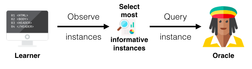
The main or core difference between an active and a passive learner is the ability to query instances based upon past queries and the responses (labels) from those queries. As you have read before, all active learning scenarios require some sort of informativeness measure of the unlabelled instances. In this section I will explain three popular approaches for querying instances under the common topic called uncertainty sampling due to its use of probabilities (for more query strategies and more in-depth information on active learning in general I recommend this survey paper).

I will use the table below to explain the query strategies. This table shows two data points (instances) and the probabilities that each instance has each label. The probability d₁ has label A, B and C is 0.9, 0.09 and 0.01 respectively and 0.2, 0.5 and 0.3 for d₂.

• Least Confidence (LC): in this strategy, the learner selects the instance for which it has the least confidence in its most likely label. Looking at the table, the leaner is pretty confident about the label for d₁, since it thinks it should be labelled A with probability 0.9, however, it is less sure about the label of d₂ since its probabilities are more spread and it thinks that it should be labelled B with a probability of only 0.5. Thus, using least confidence, the learner would select d₂ to query it's actual label.

• Margin Sampling: the shortcoming of the LC strategy, is that it only takes into consideration the most probable label and disregards the other label probabilities. The margin sampling strategy seeks to overcome this disadvantage by selecting the instance that has the smallest difference between the first and second most probable labels. Looking at d₁, the difference between its first and second most probable labels is 0.81 (0.9 - 0.09) and for d₂ it is 0.2 (0.5 - 0.3). Hence, the leaner will select d₂ again.

• Entropy Sampling: in order to utilize all the possible label probabilities, you use a popular measure called entropy. The entropy formula is applied to each instance and the instance with the largest value is queried. Using our example, d₁ has a value of 0.155 while d₂'s value is 0.447 and so the learner will select d₂ once again.

Putting it all Together

Up until now, you have read about the different components that make up active learning. It may seem a bit confusing or hard to put together all the steps but in this section, you will go through an example in full -- albeit a very simple example.

Step 0: Gather Data

This step may seem trivial, however, it is important to ensure that the dataset you gather is representative of the true distribution of the data. In other words, try to avoid a lot of skewed data. In reality it is impossible to have a totally representative sample due to limitations such as legal, time or availability.

In this example, you will have the following 5 data points. Feature A and Feature B represent some features that a data point might have. It is important to note that the data we gather is unlabelled.

Step 1: Split into Seed and Unlabelled Datasets

Next, you need to split our data into a very small dataset which we will label and a large unlabelled dataset. In active learning terminology, we call this small labelled dataset the seed. There is no set number or percentage of the unlabelled data that is typically used. Once you have set aside the data that you will use for the seed, you should label them.

Note that, in most of the literature, researchers do no use an oracle or an expert to label these instances. Typically, they get a dataset that is fully labelled and use a small amount for the seed (since they already have the label) and use the rest as if they are unlabelled. Whenever the learner selects an instance to query the orcale with, they simply just look up the label for the instance.

Continuing with the example, you select two instances for the seed, d₁ and d₃. The possible labels in this case are 'Y' and 'N'.

Seed/labelled Dataset

Unlabelled Dataset

Step 2: Train the Model

After splitting our data, you use the seed to train our learner like a normal machine learning project (using cross-validation etc.). Also, the type of learner that is used would be based on your knowledge of the domain and typically, you would use leaners that give a probabilistic response to whether an instance has a particular label, as you use these probabilities for the query strategies.

In the example, you can use any classifier you want and you will train on your two labelled instances.

Step 3: Choose unlabelled instances

Once you have trained your learner, you are now ready to select an instance or instances to query. You would have to determine the type of scenario your would like to use (that is, Membership Query Synthesis, Stream-Based Selective Sampling or Pool-Based sampling) and the query strategy.

You will use pool-based sampling with a batch size of 2. This means at each iteration, you will select two instances from your unlabelled dataset and then you add these instances to your labelled dataset. You use least confidence to select your instances. Your leaner selects d₂ and d₄ whose queried labels are 'Y' and 'N', respectively.

Labelled Dataset

Unlabelled Dataset

Step 4: Stopping criteria

Now, you can repeat steps 2 and 3 until some stopping criteria. That means that, when you have our new labelled dataset, you will re-train your leaner and then select further unlabelled data to query. One stopping criteria could be the number of instances queried, another could be the number of iterations of steps 2 and 3, you can also stop after the performance does not improve significantly above a certain threshold.

In your example, you will stop at one iteration and so you are finished with your active learning algorithm. You can also have a separate test dataset that you evaluate your learner on and record its performance. This way, you can see how your performance on the test set improved or stagnated with added labelled data.

Applications and Modern Research into Active Learning

One of the most popular areas in active learning is natural language processing (NLP). This is because many applications in NLP require lots of labelled data (for example, Part-of-Speech Tagging, Named Entity Recognition) and there is a very high cost to labelling this data.

In fact, there are only a handful datasets in NLP that are freely available and fully tagged for these applications. Hence, using active learning can significantly reduce the amount of labelled data that is needed and the experts required to accurately label them. This same reasoning can be applied to many speech recognition tasks and even tasks such as information retrieval.

Active learning is still being heavily researched. Many people have begun research into using different deep learning algorithms like CNNs and LSTMS as the learner and how to improve their efficiency when using active learning frameworks (Kronrod and Anandkumar, 2017; Sener and Savarese, 2017). There is also research being done on implementing Generative Adversarial Networks (GANs) into the active learning framework (Zhu and Bento, 2017). With the increasing interest into deep reinforcement learning, researchers are trying to reframe active learning as a reinforcement learning problem (Fang et. al, 2017). Also, there are papers which try to learn active learning strategies via a meta-learning setting (Fang et. al, 2017).