Customer Lifetime Value

Italian economist Vilfredo Pareto states that 80% of the effect comes from 20% of the causes, this is known as 80/20 rule or Pareto principle. Similarly, 80% of companies business comes from 20% customers. Companies need to identify those top customers and maintain the relationship with them to ensure continuous revenue. In order to maintain a long-term relationship with customers, companies need to schedule loyalty schemes such as the discount, offers, coupons, bonus point, and gifts.

Targeting a new customer is more costly than retaining existing customers because you don’t need to spend resources, time, and work hard to acquire new customers. You just have to keep the existing customers happy. Business analyst's accurately calculate customer acquisition cost using CLTV(Customer Lifetime Value). CLTV indicates the total revenue from the customer during the entire relationship. CLTV helps companies to focus on those potential customers who can bring in the more revenue in the future.

Customer Lifetime Value (CLTV)

"Customer Lifetime Value is a monetary value that represents the amount of revenue or profit a customer will give the company over the period of the relationship". CLTV demonstrates the implications of acquiring long-term customers compare to short-term customers. Customer lifetime value (CLV) can help you to answers the most important questions about sales to every company:

• How to Identify the most profitable customers?
• How can a company offer the best product and make the most money?
• How to segment profitable customers?
• How much budget need to spend to acquire customers?

Calculate Customer Lifetime Value

There are lots of approaches available for calculating CLTV. Everyone has his/her own view on it. For computing CLTV we need historical data of customers but you will unable to calculate for new customers. To solve this problem Business Analyst develops machine learning models to predict the CLTV of newly customers. Let's explore some approaches for CLTV Calculation:

1) You can compute it by adding profit/revenue from customers in a given cycle. For Example, If the customer is associated with you for the last 3 years, you can sum all the profit in this 3 years. You can average the profit yearly or half-yearly or monthly, but in this approach, you cannot able to build a predictive model for new customers.

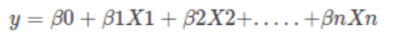
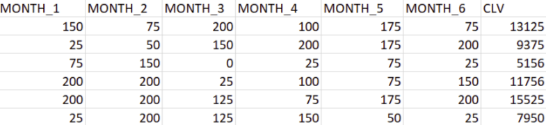
2) Build a regression model for existing customers. Take recent six-month data as independent variables and total revenue over three years as a dependent variable and build a regression model on this data.

3) CLTV can also implement using RFM(Recency, Frequency, Monetary) values. For more details, you can refer to my tutorial.

4) Using the following equation: CLTV = ((Average Order Value x Purchase Frequency)/Churn Rate) x Profit margin.

      Customer Value = Average Order Value * Purchase Frequency

• Average Order Value(AOV): The Average Order value is the ratio of your total revenue and the total number of orders. AOV represents the mean amount of revenue that the customer spends on an order.

                       Average Order Value = Total Revenue / Total Number of Orders
  

• Purchase Frequency(PF): Purchase Frequency is the ratio of the total number of orders and the total number of customer. It represents the average number of orders placed by each customer.

                      Purchase Frequency =  Total Number of Orders / Total Number of Customers
  

• Churn Rate: Churn Rate is the percentage of customers who have not ordered again.

• Customer Lifetime: Customer Lifetime is the period of time that the customer has been continuously ordering.

                                Customer Lifetime=1/Churn Rate
  

• Repeat Rate: Repeat rate can be defined as the ratio of the number of customers with more than one order to the number of unique customers. Example: If you have 10 customers in a month out of who 4 come back, your repeat rate is 40%.

                                 Churn Rate= 1-Repeat Rate
  

CLTV Implementation in Python (Using Formula)

Importing Required Library

#import modules
import pandas as pd # for dataframes
import matplotlib.pyplot as plt # for plotting graphs
import seaborn as sns # for plotting graphs
import datetime as dt
import numpy as np

Loading Dataset

Let's first load the required Online Retail dataset using the pandas read CSV function. You can download the data from here.

data = pd.read_excel("Online_Retail.xlsx")

data.head()

Removing Duplicates

Sometimes you get a messy dataset. You may have to deal with duplicates, which will skew your analysis. In python, pandas offer function drop_duplicates(), which drops the repeated or duplicate records.

filtered_data=data[['Country','CustomerID']].drop_duplicates()

Let's Jump into Data Insights

#Top ten country's customer
filtered_data.Country.value_counts()[:10].plot(kind='bar')

<matplotlib.axes._subplots.AxesSubplot at 0x7fe677a887f0>

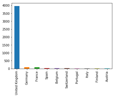
In the given dataset, you can observe most of the customers are from "United Kingdom". So, you can filter data for United Kingdom customer.

uk_data=data[data.Country=='United Kingdom']
uk_data.info()

<class 'pandas.core.frame.DataFrame'>
Int64Index: 495478 entries, 0 to 541893
Data columns (total 8 columns):
InvoiceNo      495478 non-null object
StockCode      495478 non-null object
Description    494024 non-null object
Quantity       495478 non-null int64
InvoiceDate    495478 non-null datetime64[ns]
UnitPrice      495478 non-null float64
CustomerID     361878 non-null float64
Country        495478 non-null object
dtypes: datetime64[ns](1), float64(2), int64(1), object(4)
memory usage: 34.0+ MB

The describe() function in pandas is convenient in getting various summary statistics. This function returns the count, mean, standard deviation, minimum and maximum values and the quantiles of the data.

uk_data.describe()

Here, you can observe some of the customers have ordered in a negative quantity, which is not possible. So, you need to filter Quantity greater than zero.

uk_data = uk_data[(uk_data['Quantity']>0)]
uk_data.info()

<class 'pandas.core.frame.DataFrame'>
Int64Index: 486286 entries, 0 to 541893
Data columns (total 8 columns):
InvoiceNo      486286 non-null object
StockCode      486286 non-null object
Description    485694 non-null object
Quantity       486286 non-null int64
InvoiceDate    486286 non-null datetime64[ns]
UnitPrice      486286 non-null float64
CustomerID     354345 non-null float64
Country        486286 non-null object
dtypes: datetime64[ns](1), float64(2), int64(1), object(4)
memory usage: 33.4+ MB

Filter required Columns

Here, you can filter the necessary columns for calculating CLTV. You only need her five columns CustomerID, InvoiceDate, InvoiceNo, Quantity, and UnitPrice.

• CustomerID will uniquely define your customers.
• InvoiceDate help you calculate numbers of days customer stayed with your product.
• InvoiceNo helps you to count the number of time transaction performed(frequency).
• Quantity is purchased item units in each transaction
• UnitPrice of each unit purchased by the customer will help you to calculate the total purchased amount.

uk_data=uk_data[['CustomerID','InvoiceDate','InvoiceNo','Quantity','UnitPrice']]

#Calulate total purchase
uk_data['TotalPurchase'] = uk_data['Quantity'] * uk_data['UnitPrice']

Here, you are going to perform the following operations:

• Calculate the number of days between the present date and the date of last purchase from each customer.
• Calculate the number of orders for each customer.
• Calculate sum of purchase price for each customer.

uk_data_group=uk_data.groupby('CustomerID').agg({'InvoiceDate': lambda date: (date.max() - date.min()).days,
                                        'InvoiceNo': lambda num: len(num),
                                        'Quantity': lambda quant: quant.sum(),
                                        'TotalPurchase': lambda price: price.sum()})

uk_data_group.head()

Rename the column

# Change the name of columns
uk_data_group.columns=['num_days','num_transactions','num_units','spent_money']
uk_data_group.head()

Calculate CLTV using following formula:

 CLTV = ((Average Order Value x Purchase Frequency)/Churn Rate) x Profit margin.

 Customer Value = Average Order Value * Purchase Frequency

1. Calculate Average Order Value

# Average Order Value
uk_data_group['avg_order_value']=uk_data_group['spent_money']/uk_data_group['num_transactions']

uk_data_group.head()

2. Calculate Purchase Frequency

purchase_frequency=sum(uk_data_group['num_transactions'])/uk_data_group.shape[0]

3. Calculate Repeat Rate and Churn Rate

# Repeat Rate
repeat_rate=uk_data_group[uk_data_group.num_transactions > 1].shape[0]/uk_data_group.shape[0]

#Churn Rate
churn_rate=1-repeat_rate

purchase_frequency,repeat_rate,churn_rate

(90.37107880642694, 0.9818923743942872, 0.018107625605712774)

4. Calculate Profit Margin

Profit margin is the commonly used profitability ratio. It represents how much percentage of total sales has earned as the gain. Let's assume our business has approx 5% profit on the total sale.

# Profit Margin
uk_data_group['profit_margin']=uk_data_group['spent_money']*0.05

uk_data_group.head()

5. Calcualte Customer Lifetime Value

# Customer Value
uk_data_group['CLV']=(uk_data_group['avg_order_value']*purchase_frequency)/churn_rate

#Customer Lifetime Value
uk_data_group['cust_lifetime_value']=uk_data_group['CLV']*uk_data_group['profit_margin']

uk_data_group.head()

Prediction Model for CLTV

Let's build the CLTV prediction model.

Here, you are going to predict CLTV using Linear Regression Model.

Let's first use the data loaded and filtered above.

uk_data.head()

Extract month and year from InvoiceDate.

uk_data['month_yr'] = uk_data['InvoiceDate'].apply(lambda x: x.strftime('%b-%Y'))

uk_data.head()

The pivot table takes the columns as input, and groups the entries into a two-dimensional table in such a way that provides a multidimensional summarization of the data.

sale=uk_data.pivot_table(index=['CustomerID'],columns=['month_yr'],values='TotalPurchase',aggfunc='sum',fill_value=0).reset_index()

sale.head()

Let's sum all the months sales.

sale['CLV']=sale.iloc[:,2:].sum(axis=1)

sale.head()

Selecting Feature

Here, you need to divide the given columns into two types of variables dependent(or target variable) and independent variable(or feature variables). Select latest 6 month as independent variable.

X=sale[['Dec-2011','Nov-2011', 'Oct-2011','Sep-2011','Aug-2011','Jul-2011']]
y=sale[['CLV']]

Splitting Data

To understand model performance, dividing the dataset into a training set and a test set is a good strategy.

Let's split dataset by using function train_test_split(). You need to pass 3 parameters features, target, and test_set size. Additionally, you can use random_state as a seed value to maintain reproducibility, which means whenever you split the data will not affect the results. Also, if random_state is None, then random number generator uses np.random for selecting records randomly. It means If you don't set a seed, it is different each time.

#split training set and test set
from sklearn.cross_validation import train_test_split
X_train, X_test, y_train, y_test = train_test_split(X, y,random_state=0)

Model Development

First, import the Linear Regression module and create a Linear Regression object. Then, fit your model on the train set using fit() function and perform prediction on the test set using predict() function.

# import model
from sklearn.linear_model import LinearRegression

# instantiate
linreg = LinearRegression()

# fit the model to the training data (learn the coefficients)
linreg.fit(X_train, y_train)

# make predictions on the testing set
y_pred = linreg.predict(X_test)

# print the intercept and coefficients
print(linreg.intercept_)
print(linreg.coef_)

[208.50969617]
[[0.99880551 0.80381254 1.60226829 1.67433228 1.52860813 2.87959449]]

How Well Does the Model Fit the data?

In order to evaluate the overall fit of the linear model, we use the R-squared value. R-squared is the proportion of variance explained by the model. Value of R-squared lies between 0 and 1. Higher value or R-squared is considered better because it indicates the larger variance explained by the model.

from sklearn import metrics

# compute the R Square for model
print("R-Square:",metrics.r2_score(y_test, y_pred))

R-Square: 0.9666074402817512

This model has a higher R-squared (0.96). This model provides a better fit to the data.

Model Evaluation

For regression problems following evaluation metrics used (Ritchie Ng):

• Mean Absolute Error (MAE) is the mean of the absolute value of the errors.
• Mean Squared Error (MSE) is the mean of the squared errors.
• Root Mean Squared Error (RMSE) is the square root of the mean of the squared errors.

# calculate MAE using scikit-learn
print("MAE:",metrics.mean_absolute_error(y_test,y_pred))

#calculate mean squared error
print("MSE",metrics.mean_squared_error(y_test, y_pred))
# compute the RMSE of our predictions
print("RMSE:",np.sqrt(metrics.mean_squared_error(y_test, y_pred)))

MAE: 595.0282284701234
MSE 2114139.8898678957
RMSE: 1454.0082151995896

RMSE is more popular than MSE and MAE because RMSE is interpretable with y because of the same units.

Pros and Cons of CLTV

CLTV helps you to design an effective business plan and also provide a chance to scale your business. CLTV draw meaningful customer segments these segment can help you to identify needs of the different-different segment.

Customer Lifetime Value is a tool, not a strategy. CLTV can figure out most profitable customers, but how you are going to make a profit from them, it depends on your strategy. Generally, CLTV models are confused and misused. Obsession with CLTV may create blinders. Companies only focus on finding the best customer group and focusing on them and repeat the business, but it’s also important to give attention to other customers.

Conclusion

Congratulations, you have made it to the end of this tutorial!

In this tutorial, you have covered a lot of details about Customer Lifetime Value. You have learned what customer lifetime value is, approaches for calculating CLTV, implementation of CLTV from scratch in python, a prediction model for CLTV, and Pros and Cons of CLTV. Also, you covered some basic concepts of pandas such as groupby and pivot table for summarizing selected columns and rows of data.

Hopefully, you can now utilize CLTV concept to analyze your own datasets. Thanks for reading this tutorial!

If you would like to learn more about analyzing customer data in Python, take DataCamp's Customer Analytics & A/B Testing in Python course.