Five Tips to Improve your R Code

3. Ditch the which()

Next time you use which(), try to ditch it! People often use which() to get indices from some boolean condition, and then select values at those indices. This is not necessary.

Getting vector elements greater than 5:

x <- 3:7

# Using which (not necessary)
x[which(x > 5)]
#> [1] 6 7

# No which
x[x > 5]
#> [1] 6 7

Or counting number of values greater than 5:

# Using which
length(which(x > 5))
#> [1] 2

# Without which
sum(x > 5)
#> [1] 2

Why should you ditch which()? It's often unnecessary and boolean vectors are all you need.

For example, R lets you select elements flagged as TRUE in a boolean vector:

condition <- x > 5
condition
#> [1] FALSE FALSE FALSE  TRUE  TRUE
x[condition]
#> [1] 6 7

Also, when combined with sum() or mean(), boolean vectors can be used to get the count or proportion of values meeting a condition:

sum(condition)
#> [1] 2
mean(condition)
#> [1] 0.4

which() tells you the indices of TRUE values:

which(condition)
#> [1] 4 5

And while the results are not wrong, it's just not necessary. For example, I often see people combining which() and length() to test whether any or all values are TRUE. Instead, you just need any() or all():

x <- c(1, 2, 12)

# Using `which()` and `length()` to test if any values are greater than 10
if (length(which(x > 10)) > 0)
  print("At least one value is greater than 10")
#> [1] "At least one value is greater than 10"

# Wrapping a boolean vector with `any()`
if (any(x > 10))
  print("At least one value is greater than 10")
#> [1] "At least one value is greater than 10"

# Using `which()` and `length()` to test if all values are positive
if (length(which(x > 0)) == length(x))
  print("All values are positive")
#> [1] "All values are positive"

# Wrapping a boolean vector with `all()`
if (all(x > 0))
  print("All values are positive")
#> [1] "All values are positive"

Oh, and it saves you a little time...

x <- runif(1e8)

system.time(x[which(x > .5)])
#>    user  system elapsed 
#>   1.156   0.522   1.686

system.time(x[x > .5])
#>    user  system elapsed 
#>   1.071   0.442   1.662

4. factor that factor!

Ever removed values from a factor and found you're stuck with old levels that don't exist anymore? I see all sorts of creative ways to deal with this. The simplest solution is often just to wrap it in factor() again.

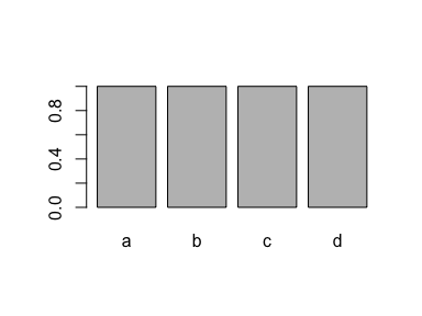
This example creates a factor with four levels ("a", "b", "c" and "d"):

# A factor with four levels
x <- factor(c("a", "b", "c", "d"))
x
#> [1] a b c d
#> Levels: a b c d

plot(x)

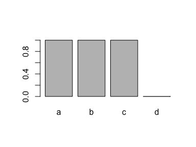
If you drop all cases of one level ("d"), the level is still recorded in the factor:

# Drop all values for one level
x <- x[x != "d"]

# But we still have this level!
x
#> [1] a b c
#> Levels: a b c d

plot(x)

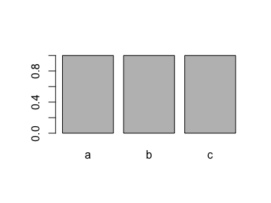
A super simple method for removing it is to use factor() again:

x <- factor(x)
x
#> [1] a b c
#> Levels: a b c

plot(x)

This is typically a good solution to a problem that gets a lot of people mad. So save yourself a headache and factor that factor!

5. First you get the $, then you get the power

Next time you want to extract values from a data.frame column where the rows meet a condition, specify the column with $ before the rows with [.

Say you want the horsepower (hp) for cars with 4 cylinders (cyl), using the mtcars data set. You can write either of these:

# rows first, column second - not ideal
mtcars[mtcars$cyl == 4, ]$hp
#>  [1]  93  62  95  66  52  65  97  66  91 113 109

# column first, rows second - much better
mtcars$hp[mtcars$cyl == 4]
#>  [1]  93  62  95  66  52  65  97  66  91 113 109

The tip here is to use the second approach.

But why is that?

First reason: do away with that pesky comma! When you specify rows before the column, you need to remember the comma: mtcars[mtcars$cyl == 4,]$hp. When you specify column first, this means that you're now referring to a vector, and don't need the comma!

Second reason: speed! Let's test it out on a larger data frame:

# Simulate a data frame...
n <- 1e7
d <- data.frame(
  a = seq(n),
  b = runif(n)
)

# rows first, column second - not ideal
system.time(d[d$b > .5, ]$a)
#>    user  system elapsed 
#>   0.497   0.126   0.629

# column first, rows second - much better
system.time(d$a[d$b > .5])
#>    user  system elapsed 
#>   0.089   0.017   0.107

Worth it, right?

Still, if you want to hone your skills as an R data frame ninja, I suggest learning dplyr. You can get a good overview on the dplyr website or really learn the ropes with online courses like DataCamp's Data Manipulation in R with dplyr.

Sign off

Thanks for reading and I hope this was useful for you.

For updates of recent blog posts, follow @drsimonj on Twitter, or email me at [email protected] to get in touch.

If you'd like the code that produced this blog, check out the blogR GitHub repository.

Check out our Getting Started with the Tidyverse: Tutorial.