Support Vector Machines in R

In machine learning, support vector machines are supervised learning models with associated learning algorithms that analyze data used for classification and regression analysis. However, they are mostly used in classification problems. In this tutorial, we will try to gain a high-level understanding of how SVMs work and then implement them using R. I’ll focus on developing intuition rather than rigor. What that essentially means is we will skip as much of the math as possible and develop a strong intuition of the working principle.

Support Vector Machines Algorithm

Linear Data

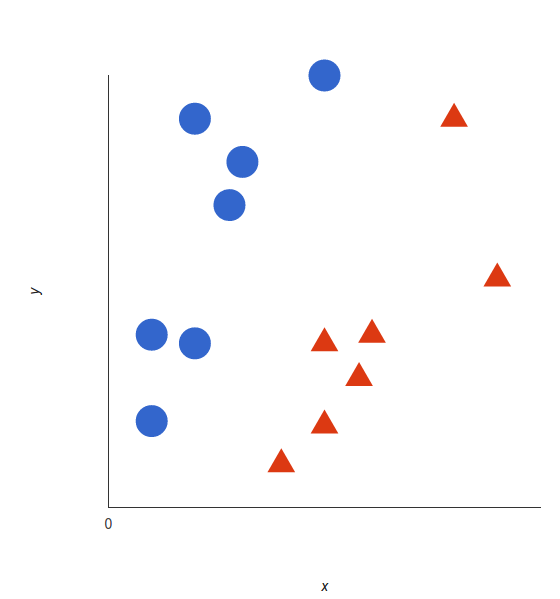
The basics of Support Vector Machines and how it works are best understood with a simple example. Let’s imagine we have two tags: red and blue, and our data has two features: x and y. We want a classifier that, given a pair of (x,y) coordinates, outputs if it’s either red or blue. We plot our already labeled training data on a plane:

A support vector machine takes these data points and outputs the hyperplane (which in two dimensions it’s simply a line) that best separates the tags. This line is the decision boundary: anything that falls to one side of it we will classify as blue, and anything that falls to the other as red.

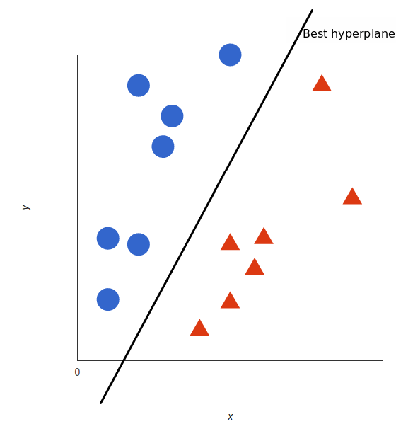
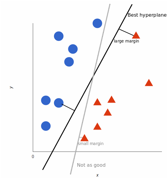
But, what exactly is the best hyperplane? For SVM, it’s the one that maximizes the margins from both tags. In other words: the hyperplane (remember it’s a line in this case) whose distance to the nearest element of each tag is the largest.

Non-Linear Data

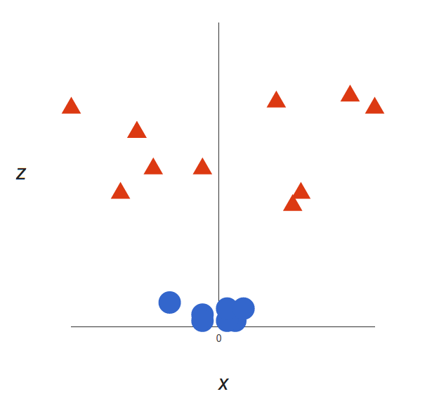
Now the example above was easy since clearly, the data was linearly separable — we could draw a straight line to separate red and blue. Sadly, usually things aren’t that simple. Take a look at this case:

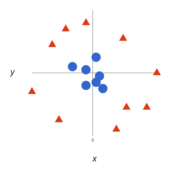
It’s pretty clear that there’s not a linear decision boundary (a single straight line that separates both tags). However, the vectors are very clearly segregated, and it looks as though it should be easy to separate them.

So here’s what we’ll do: we will add a third dimension. Up until now, we had two dimensions: $x$ and $y$. We create a new z dimension, and we rule that it be calculated a certain way that is convenient for us: $z = x² + y²$ (you’ll notice that’s the equation for a circle).

This will give us a three-dimensional space. Taking a slice of that space, it looks like this:

What can SVM do with this? Let’s see:

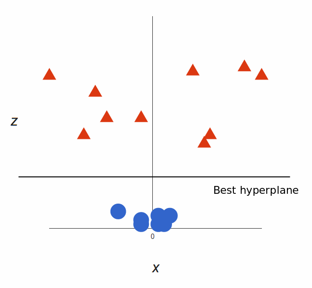
That’s great! Note that since we are in three dimensions now, the hyperplane is a plane parallel to the $x$ axis at a certain $z$ (let’s say $z = 1$).

What’s left is mapping it back to two dimensions:

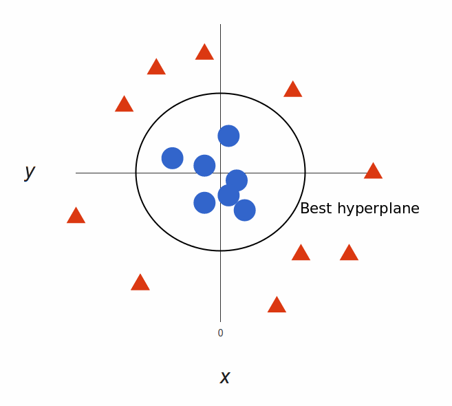
And there we go! Our decision boundary is a circumference of radius 1, which separates both tags using SVM.

Kernel Trick

In the above example, we found a way to classify nonlinear data by cleverly mapping our space to a higher dimension. However, it turns out that calculating this transformation can get pretty computationally expensive: there can be a lot of new dimensions, each one of them possibly involving a complicated calculation. Doing this for every vector in the dataset can be a lot of work, so it’d be great if we could find a cheaper solution.

Here’s a trick: SVM doesn’t need the actual vectors to work its magic, it actually can get by only with the dot products between them. This means that we can sidestep the expensive calculations of the new dimensions! This is what we do instead:

• Imagine the new space we want:

• Figure out what the dot product in that space looks like:

• Tell SVM to do its thing, but using the new dot product — we call this a kernel function.

This is known as the kernel trick, which enlarges the feature space in order to accommodate a non-linear boundary between the classes. Common types of kernels used to separate non-linear data are polynomial kernels, radial basis kernels, and linear kernels (which are the same as support vector classifiers). Simply, these kernels transform our data to pass a linear hyperplane and thus classify our data.

Advantages and Disadvantages

Let us now look at some advantages and disadvantages of SVM:

Advantages

• High Dimensionality: SVM is an effective tool in high-dimensional spaces, which is particularly applicable to document classification and sentiment analysis where the dimensionality can be extremely large.

• Memory Efficiency: Since only a subset of the training points are used in the actual decision process of assigning new members, just these points need to be stored in memory (and calculated upon) when making decisions.

• Versatility: Class separation is often highly non-linear. The ability to apply new kernels allows substantial flexibility for the decision boundaries, leading to greater classification performance.

Disadvantages

• Kernel Parameters Selection: SVMs are very sensitive to the choice of the kernel parameters. In situations where the number of features for each object exceeds the number of training data samples, SVMs can perform poorly. This can be seen intuitively as if the high-dimensional feature space is much larger than the samples. Then there are less effective support vectors on which to support the optimal linear hyperplanes, leading to poorer classification performance as new unseen samples are added.

• Non-Probabilistic: Since the classifier works by placing objects above and below a classifying hyperplane, there is no direct probabilistic interpretation for group membership. However, one potential metric to determine the "effectiveness" of the classification is how far from the decision boundary the new point is.

Support Vector Machines in R

Linear SVM Classifier

Let's first generate some data in 2 dimensions, and make them a little separated. After setting random seed, you make a matrix x, normally distributed with 20 observations in 2 classes on 2 variables. Then you make a y variable, which is going to be either -1 or 1, with 10 in each class. For y = 1, you move the means from 0 to 1 in each of the coordinates. Finally, you can plot the data and color code the points according to their response. The plotting character 19 gives you nice big visible dots coded blue or red according to whether the response is 1 or -1.

set.seed(10111)
x = matrix(rnorm(40), 20, 2)
y = rep(c(-1, 1), c(10, 10))
x[y == 1,] = x[y == 1,] + 1
plot(x, col = y + 3, pch = 19)

Now you load the package e1071 which contains the svm function (remember to install the package if you haven't already).

library(e1071)

Now you make a dataframe of the data, turning y into a factor variable. After that, you make a call to svm on this dataframe, using y as the response variable and other variables as the predictors. The dataframe will have unpacked the matrix x into 2 columns named x1 and x2. You tell SVM that the kernel is linear, the tune-in parameter cost is 10, and scale equals false. In this example, you ask it not to standardize the variables.

dat = data.frame(x, y = as.factor(y))
svmfit = svm(y ~ ., data = dat, kernel = "linear", cost = 10, scale = FALSE)
print(svmfit)

Printing the svmfit gives its summary. You can see that the number of support vectors is 6 - they are the points that are close to the boundary or on the wrong side of the boundary.

There's a plot function for SVM that shows the decision boundary, as you can see below. It doesn't seem there's much control over the colors. It breaks with convention since it puts x2 on the horizontal axis and x1 on the vertical axis.

plot(svmfit, dat)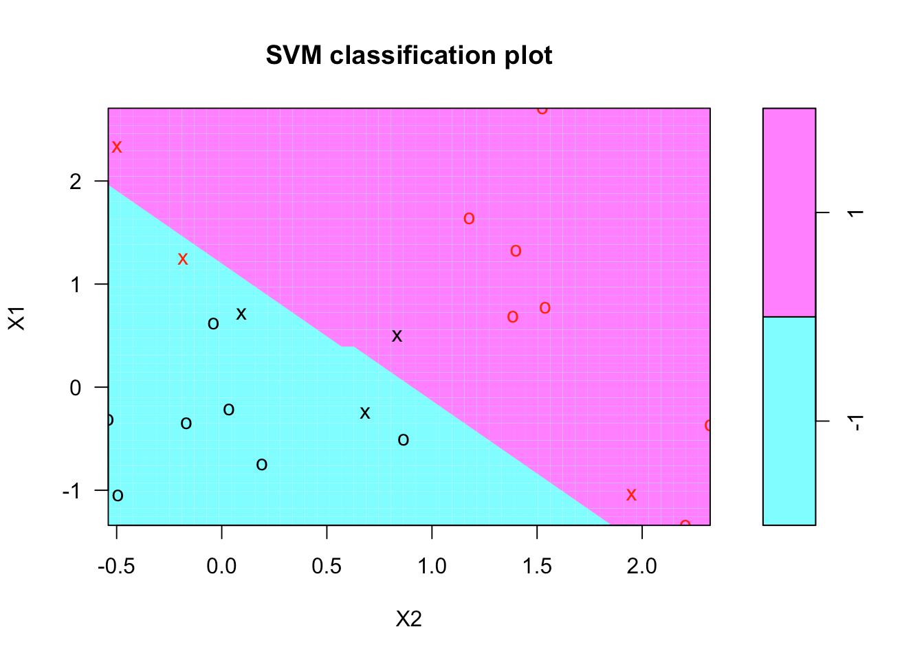

Let's try to make your own plot. The first thing to do is to create a grid of values or a lattice of values for x1 and x2 that covers the whole domain on a fairly fine lattice. To do so, you make a function called make.grid. It takes in your data matrix x, as well as an argument n which is the number of points in each direction. Here you're going to ask for a 75 x 75 grid.

Within this function, you use the apply function to get the range of each of the variables in x. Then for both x1 and x2, you use the seq function to go from the lowest value to the upper value to make a grid of length n. As of now, you have x1 and x2, each with length 75 uniformly-spaced values on each of the coordinates. Finally, you use the function expand.grid, which takes x1 and x2 and makes the lattice.

make.grid = function(x, n = 75) {
  grange = apply(x, 2, range)
  x1 = seq(from = grange[1,1], to = grange[2,1], length = n)
  x2 = seq(from = grange[1,2], to = grange[2,2], length = n)
  expand.grid(X1 = x1, X2 = x2)
}

Now you can apply the make.grid function on x. Let's take a look at the first few values of the lattice from 1 to 10.

xgrid = make.grid(x)
xgrid[1:10,]

As you can see, the grid goes through the 1st coordinate first, holding the 2nd coordinate fixed.

Having made the lattice, you're going to make a prediction at each point in the lattice. With the new data xgrid, you use predict and call the response ygrid. You then plot and color code the points according to the classification so that the decision boundary is clear. Let's also put the original points on this plot using the points function.

svmfit has a component called index that tells which are the support points. You include them in the plot by using the points function again.

ygrid = predict(svmfit, xgrid)
plot(xgrid, col = c("red","blue")[as.numeric(ygrid)], pch = 20, cex = .2)
points(x, col = y + 3, pch = 19)
points(x[svmfit$index,], pch = 5, cex = 2)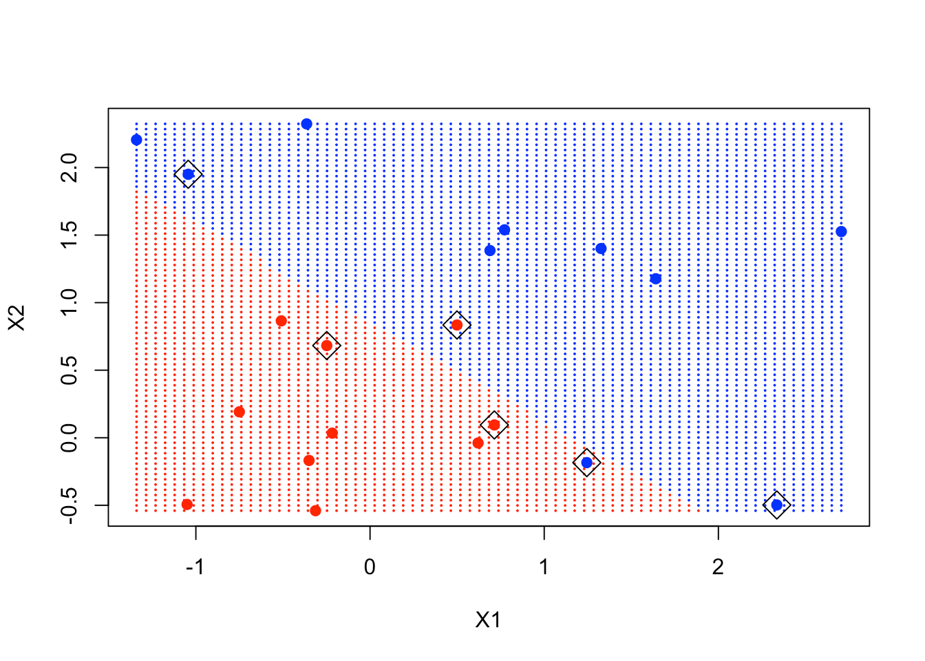

As you can see in the plot, the points in the boxes are close to the decision boundary and are instrumental in determining that boundary.

Unfortunately, the svm function is not too friendly, in that you have to do some work to get back the linear coefficients. The reason is probably that this only makes sense for linear kernels, and the function is more general. So let's use a formula to extract the coefficients more efficiently. You extract beta and beta0, which are the linear coefficients.

beta = drop(t(svmfit$coefs)%*%x[svmfit$index,])
beta0 = svmfit$rho

Now you can replot the points on the grid, then put the points back in (including the support vector points). Then you can use the coefficients to draw the decision boundary using a simple equation of the form:

From that equation, you have to figure out a slope and an intercept for the decision boundary. Then you can use the function abline with those 2 arguments. The subsequent 2 abline function represent the upper margin and the lower margin of the decision boundary, respectively.

plot(xgrid, col = c("red", "blue")[as.numeric(ygrid)], pch = 20, cex = .2)
points(x, col = y + 3, pch = 19)
points(x[svmfit$index,], pch = 5, cex = 2)
abline(beta0 / beta[2], -beta[1] / beta[2])
abline((beta0 - 1) / beta[2], -beta[1] / beta[2], lty = 2)
abline((beta0 + 1) / beta[2], -beta[1] / beta[2], lty = 2)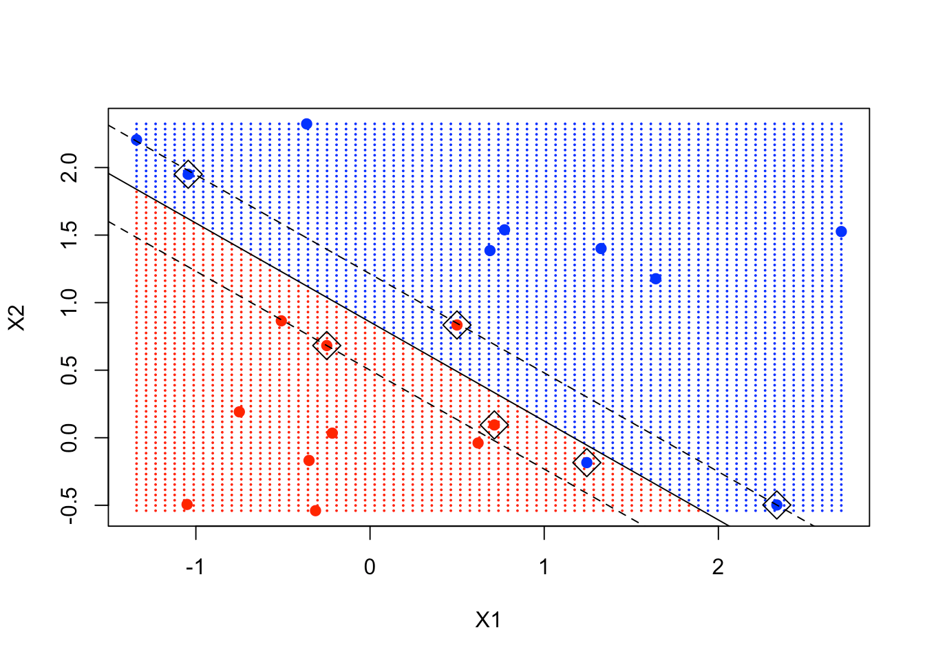

You can see clearly that some of the support points are exactly on the margin, while some are inside the margin.

Non-Linear SVM Classifier

So that was the linear SVM in the previous section. Now let's move on to the non-linear version of SVM. You will take a look at an example from the textbook Elements of Statistical Learning, which has a canonical example in 2 dimensions where the decision boundary is non-linear. You're going to use the kernel support vector machine to try and learn that boundary.

First, you get the data for that example from the textbook by downloading it directly from this URL, which is the webpage where the data reside. The data is mixed and simulated. Then you can inspect its column names.

load(file = "ESL.mixture.rda")
names(ESL.mixture)

For the moment, the training data are x and y. You've already created and x and y for the previous example. Thus, let's get rid of those so that you can attach this new data.

rm(x, y)
attach(ESL.mixture)

The data are also 2-dimensional. Let's plot them to get a good look.

plot(x, col = y + 1)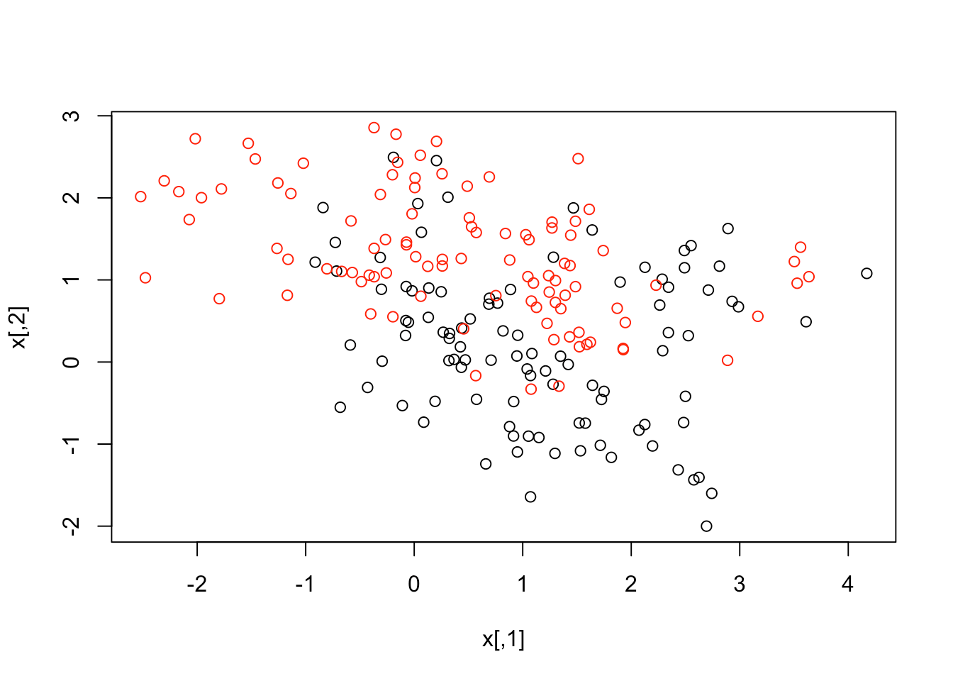

The data seems to overlap quite a bit, but you can see that there's something special in its structure. Now, let's make a data frame with the response y, and turn that into a factor. After that, you can fit an SVM with radial kernel and cost as 5.

dat = data.frame(y = factor(y), x)
fit = svm(factor(y) ~ ., data = dat, scale = FALSE, kernel = "radial", cost = 5)

It's time to create a grid and make your predictions. These data actually came supplied with grid points. If you look down on the summary on the names that were on the list, there are 2 variables px1 and px2, which are the grid of values for each of those variables. You can use expand.grid to create the grid of values. Then you predict the classification at each of the values on the grid.

xgrid = expand.grid(X1 = px1, X2 = px2)
ygrid = predict(fit, xgrid)

Finally, you plot the points and color them according to the decision boundary. You can see that the decision boundary is non-linear. You can put the data points in the plot as well to see where they lie.

plot(xgrid, col = as.numeric(ygrid), pch = 20, cex = .2)
points(x, col = y + 1, pch = 19)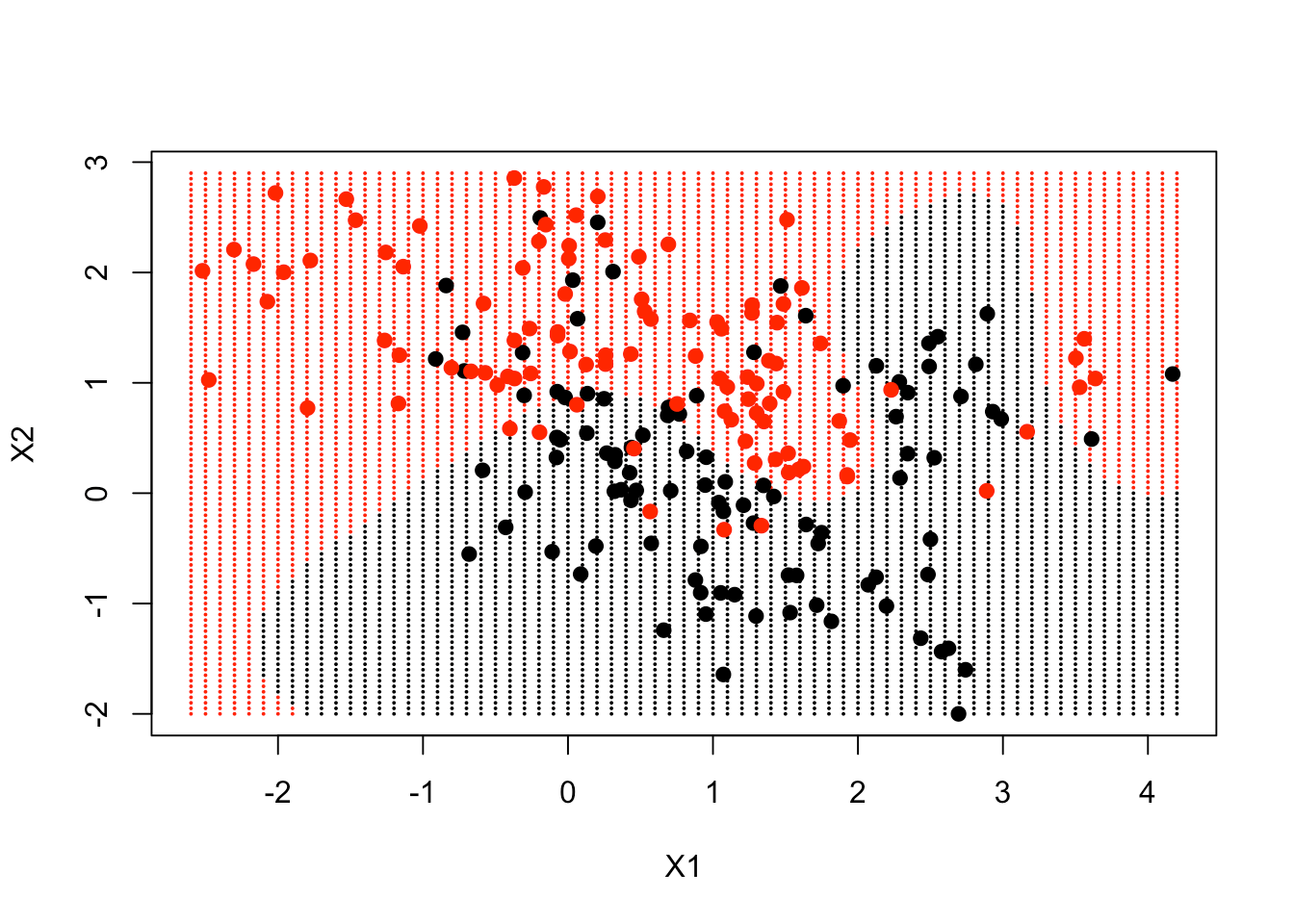

The decision boundary, to a large extent, follows where the data is, but in a very non-linear way.

Let's see if you can improve this plot a little bit further and have the predict function produce the actual function estimates at each of our grid points. In particular, you'd like to put in a curve that gives the decision boundary by making use of the contour function. On the data frame, there's also a variable called prob, which is the true probability of class 1 for these data, at the grid points. If you plot its 0.5 contour, that will give the Bayes Decision Boundary, which is the best one could ever do.

First, you predict your fit on the grid. You tell it decision values equal TRUE because you want to get the actual function, not just the classification. It returns an attribute of the actual classified values, so you have to pull of that attribute. Then you access the one called decision.

Next, you can follow the same steps as above to create the grid, make the predictions, and plot the points.

Then, it's time to use the contour function. It requires the 2 grid sequences, a function, and 2 arguments level and add. You want the function in the form of a matrix, with the dimensions of px1 and px2 (69 and 99 respectively). You set level equals 0 and add it to the plot. As a result, you can see that the contour tracks the decision boundary, a convenient way of plotting a non-linear decision boundary in 2 dimensions.

Finally, you include the truth, which is the contour of the probabilities. That's the 0.5 contour, which would be the decision boundary in terms of the probabilities (also known as the Bayes Decision Boundary).

func = predict(fit, xgrid, decision.values = TRUE)
func = attributes(func)$decision

xgrid = expand.grid(X1 = px1, X2 = px2)
ygrid = predict(fit, xgrid)
plot(xgrid, col = as.numeric(ygrid), pch = 20, cex = .2)
points(x, col = y + 1, pch = 19)

contour(px1, px2, matrix(func, 69, 99), level = 0, add = TRUE)
contour(px1, px2, matrix(func, 69, 99), level = 0.5, add = TRUE, col = "blue", lwd = 2)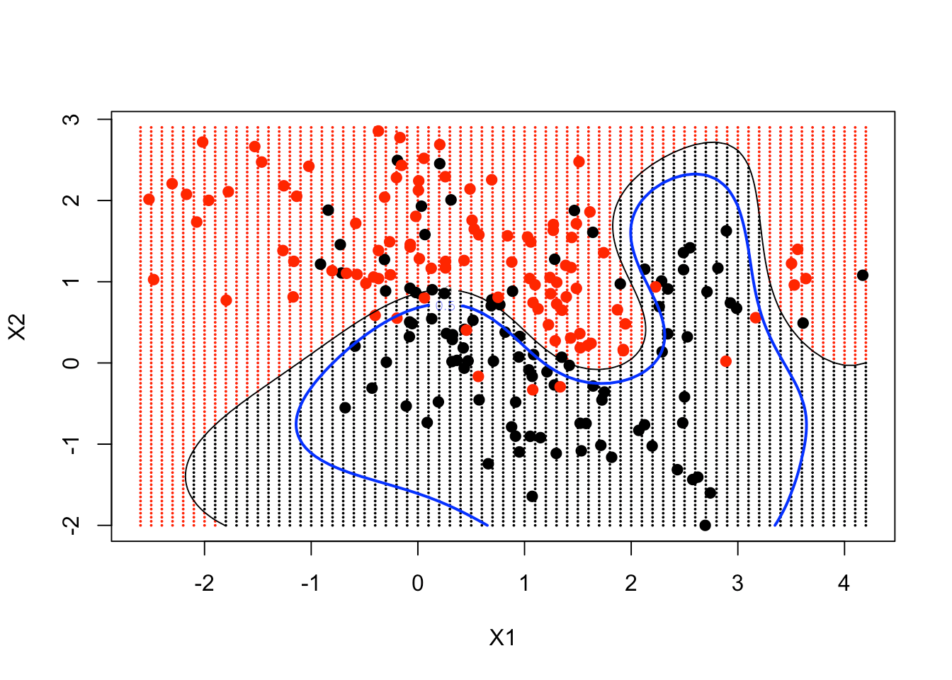

As a result, you can see your non-linear SVM has got pretty close to the Bayes Decision Boundary.

Conclusion

So to recap, Support Vector Machines are a subclass of supervised classifiers that attempt to partition a feature space into two or more groups. They achieve this by finding an optimal means of separating such groups based on their known class labels:

• In simpler cases the separation "boundary" is linear, leading to groups that are split up by lines (or planes) in high-dimensional spaces.
• In more complicated cases (where groups are not nicely separated by lines or planes), SVMs are able to carry out non-linear partitioning. This is achieved by means of a kernel function.
• Ultimately, this makes them very sophisticated and capable classifiers, but at the usual expense that they can be prone to overfitting.

Personally, I think SVMs are great classifiers for specific situations when the groups are clearly separated. They also do a great job when your data is non-linearly separated. You could transform data to linearly separate it, or you can have SVMs convert the data and linearly separate the two classes right out of the box. This is one of the main reasons to use SVMs. You don’t have to transform non-linear data yourself. One downside to SVMs is the black box nature of these functions. The use of kernels to separate non-linear data makes them difficult (if not impossible) to interpret. Understanding them will give you an alternative to GLMs and decision trees for classification. I hope this tutorial gives you a broader view of the SVM panorama and will allow you to understand these machines better.

If you would like to learn more about R, take DataCamp's Machine Learning Toolbox course.

Check out our Support Vector Machines with Scikit-learn Tutorial.