Introduction to Non-Linear Models and Insights Using R

This tutorial is a valued contribution from our community and has been edited for clarity and accuracy by DataCamp.

Interested in sharing your own expertise? We’d love to hear from you! Feel free to submit your articles or ideas through our Community Contribution Form.

Non-linear models are no longer as popular as they used to be. Today, many books skip any discussion on non-linear models or explain it in a limited capacity. Apparently, there are a good number of reasons for this. Firstly, one can fit a non-linear curve using linear regression by either using higher-order polynomial terms or applying a basis function (in other words, apply a log or sqrt transformation on the explanatory variables). Secondly, one may choose simplicity over complex models as linear models are easy to interpret and explain.

Furthermore, in order to apply a non-linear model, it is important to visualize the data and get a sense of trajectory, which is not possible in a multivariate setting. Lastly, non-linear models are best suited for mechanistic cases where the phenomena are purely physical or in deterministic terms, which is not the case for big data, where the user activities are logged by machines.

However, despite all these good reasons, non-linear modeling is a beautiful science that should be explored and compared with its linear counterpart.

Non-Linear Regression Model

The estimation techniques for a non-linear model are explicitly iterative. Additionally, there is a fundamental difference in the way one applies a non-linear formula, which is not the same as a linear formula. Following three different equations/formulas, each one is considered linear because the relation between variable y and B₀, B₁, and B₂ is a straight line.

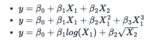
What makes a formula non-linear is something like this:

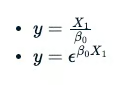
The use of B₀ or B₁ is arbitrary. However, the latter two equations do not have a straight-line relation between variable y and B₀.

Unfortunately, this makes the computations more difficult, and a successful numerical solution to the estimation problem will not be guaranteed. So, non-linear models come with a cautionary warning that getting answers out may not be intuitive or accurate.

Specialized Model

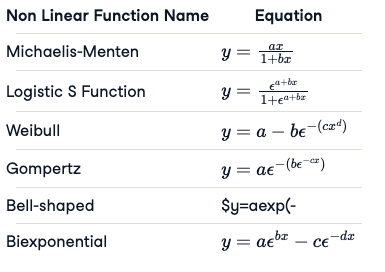
Usually, when one applies a non-linear model, they use specialized types. This makes fitting a non-linear model more convenient or numerically easier, but it needs to be agreed on by some subject matter expert and aligned with the data. By specialized types, we mean one uses a predefined mathematical equation. Here is the list of most frequently used non-linear equations (some were omitted for brevity).

Strategy Involved for Non-Linear Regression Model

1. Visualize the data to see if a specialized mathematical function can best explain the data.
2. Either eyeballing the plot or using a self-starter function (explained below), select the initial parameter values.
3. Fit the model and examine it.
4. Perform a statistical analysis on the fitted model to understand the parameter confidence interval, residual error, and the variation explained.
5. Try to add more parameters to the model if it helps to reduce the residual error.
6. Always fit a linear model and compare the results of non-linear and linear models.

Explaining the Non-Linear Model Through an Example

We are going to fit a specialized non-linear model on a popular dataset, Puromycin, which presents the reaction rate and the concentration information for an enzymatic reaction involving cells with Puromycin drug. The data comes with two classes of cells, one treated with the drug Puromycin and the other one without this drug.

names(Puromycin)
Puromycin

'conc''rate''state'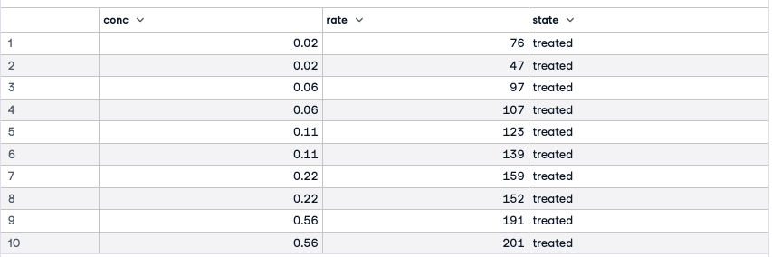

The three variables in this dataframe are the concentration of the substrate, the initial rate of the reaction, and an indicator of treated or untreated.

By plotting the rate against concentration and labeling the two levels of the treatment, we can see a general pattern. The curves are asymptotic and quite distinct for treated and untreated cell cohorts.

plot(Puromycin$conc, Puromycin$rate, type="n", xlab = "conc", ylab = "rate")
text(Puromycin$conc, Puromycin$rate, 
     ifelse(Puromycin$state == "treated", "T", "U"))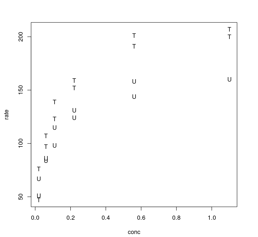

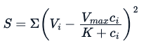
Because this data exhibits a strong Michaelis-Menten relation between the reaction rate and the concentration, the experimenters expect to fit the following mathematical equation.

Here, the E is the experimentation error. Using the same analogy used for the linear model, through a non-linear specialized model, we try to estimate parameters Vmax and K that will minimize the sum of squares of the residuals (however, there are other methods one can use to these estimate parameters):

Fitting a Non-Linear Model

Even though we know the relationship, fitting a non-linear model is not that straightforward because the model requires initial guesses for V_max and K . If one fails to not choose a good initial guess, the model may fit the data poorly. One has two options to choose from:

• Either eyeball the plot to find the initial values.
• Or use a self-starter function (given below).

For each model type, we have a corresponding self-starter function that can be used for an initial guess.

Fit a Model using an Initial Guess

Using the initial value of Vmax = 160, K = 0.05 found by eyeballing the plot, one can use the R function nls() to fit the data. Usually, for linear regression, we do not need to specify the parameters Vm or K, but it is different for a non-linear model. Every iterative algorithm needs a good starting point. Otherwise, it may fail to converge. This is how we fit in a non-linear model on Puromycin with initial values.

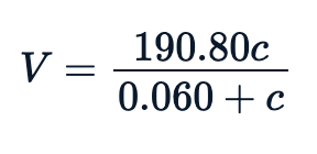
Purboth_1 <- nls(rate ~ (Vm)*conc/(K+conc), Puromycin, list(Vm=160, K=0.05))

summary(Purboth_1)

Formula: rate ~ (Vm) * conc/(K + conc)

Parameters:

Estimate Std. Error t value Pr(>|t|)

Vm 190.80624 8.76459 21.770 6.84e-16 ***

K 0.06039 0.01077 5.608 1.45e-05 ***

---

Signif. codes: 0 ‘***’ 0.001 ‘**’ 0.01 ‘*’ 0.05 ‘.’ 0.1 ‘ ’ 1

Residual standard error: 18.61 on 21 degrees of freedom

Number of iterations to convergence: 5

Achieved convergence tolerance: 5.121e-06

Calculate residual error

We calculate the residual error as:

sse <- Purboth_1$m$deviance()
sse

7276.54697931423

Calculate the variance explained

In order to find the variance explained by this model (basically R-square in the linear model terminology), we need to find the total variance in rate by fitting a null model, estimating the overall mean, and extracting the total sums of squares, sst, from the null model summary and then use it to calculate the percentage of variance explained.

sse <- Purboth_1$m$deviance()
null <- lm(rate~1, Puromycin)
sst <- data.frame(summary.aov(null)[[1]])$Sum.Sq
percent_variation_explained = 100*(sst-sse)/sst
percent_variation_explained

85.3488323994681

This model explains 85.34% of the variations in the data.

Fit using Model using Self-Start Function

Because we are using the Michaelis-Menten model, one can use SSmicmen() self-start function instead. However, this gives the same results.

Purboth_self <- nls(rate~SSmicmen(conc,Vm,K), Puromycin)
summary(Purboth_self)

Formula: rate ~ SSmicmen(conc, Vm, K)
Parameters:
Estimate Std. Error t value Pr(>|t|)
Vm 190.80667 8.76462 21.770 6.84e-16 ***
K 0.06039 0.01077 5.608 1.45e-05 ***
---
Signif. codes: 0 ‘***’ 0.001 ‘**’ 0.01 ‘*’ 0.05 ‘.’ 0.1 ‘ ’ 1
Residual standard error: 18.61 on 21 degrees of freedom
Number of iterations to convergence: 4
Achieved convergence tolerance: 6.745e-06

Calculate residual error

sse <- Purboth_self$m$deviance()
sse

7276.54697947673

Calculate the Variance Explained

One can check the variance explained by the model.

sse <- Purboth_self$m$deviance()
null <- lm(rate~1, Puromycin)
sst <- data.frame(summary.aov(null)[[1]])$Sum.Sq
percent_variation_explained = 100*(sst-sse)/sst
percent_variation_explained

85.348832399141

In general, the fitted equation, which is the relation between rate vs concentration, looks like this:

Visualizing the Fit

One can visualize how the model performs by plotting a fitted line on the data, which looks non-linear.

plot(Puromycin$conc, Puromycin$rate, xlab="conc", ylab = "rate")
lines(Puromycin[Puromycin$state == "treated",]$conc, 
      predict(Purboth_1, Puromycin[Puromycin$state == "treated",]), col=2)
lines(Puromycin[Puromycin$state != "treated",]$conc, 
      predict(Purboth_1, Puromycin[Puromycin$state != "treated",]), col=2)

Better Model Selection

One can further tune the model by adding more parameters. If one observes the plot between the rate vs concentration one may notice that different classes (treated vs untreated) follow different trajectories, and the rate difference (y-axis) between two class trajectories can be approximated as 40.

plot(Puromycin$conc, Puromycin$rate, type="n", xlab = "conc", ylab = "rate")
text(Puromycin$conc, Puromycin$rate, 
     ifelse(Puromycin$state == "treated", "+", "*"))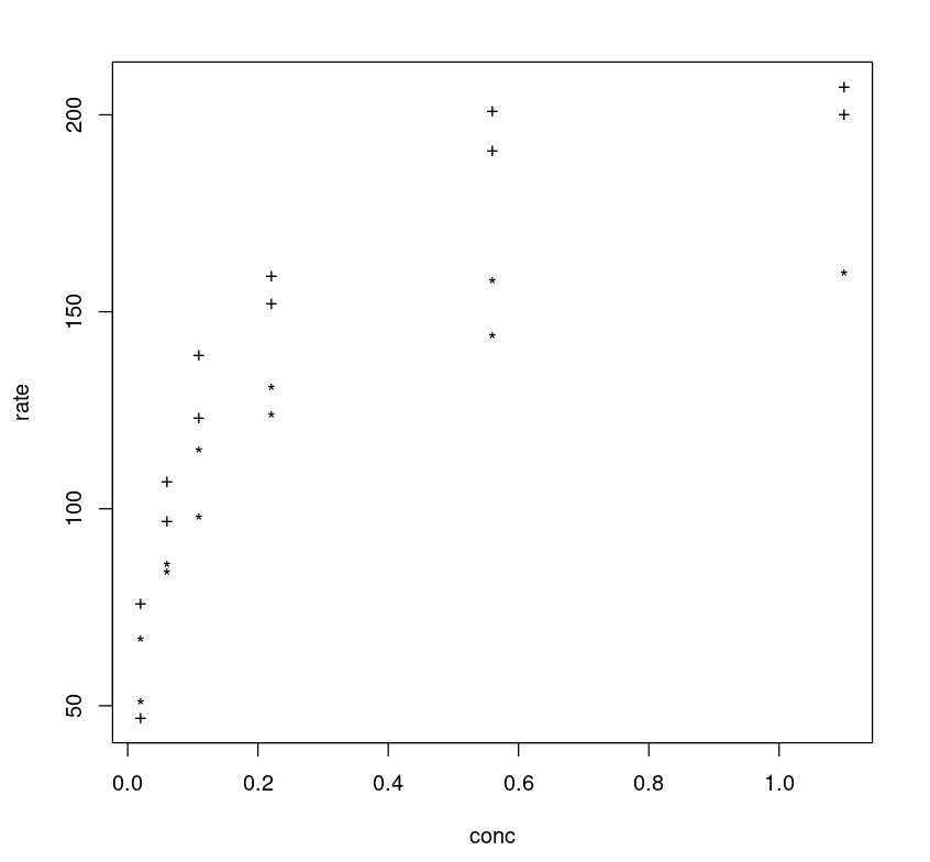

Essentially, we are trying to fit a model conditioning on the state variable, which leads to the following non-linear equation.

The model performs better with an additional parameter delV. We assign an initial value of 40 to delV and fit the model using nls with three parameters.

Purboth <- nls(rate ~ (Vm + delV*(state=="treated"))*conc/(K+conc), Puromycin, 
               list(Vm=160, delV=40, K=0.05))
summary(Purboth)

Formula: rate ~ (Vm + delV * (state == "treated")) * conc/(K + conc)

Parameters:
      Estimate Std. Error t value Pr(>|t|)    
Vm   166.60397    5.80742  28.688  < 2e-16 ***
delV  42.02591    6.27214   6.700 1.61e-06 ***
K      0.05797    0.00591   9.809 4.37e-09 ***
---
Signif. codes:  0 ‘***’ 0.001 ‘**’ 0.01 ‘*’ 0.05 ‘.’ 0.1 ‘ ’ 1

Residual standard error: 10.59 on 20 degrees of freedom

Number of iterations to convergence: 5 
Achieved convergence tolerance: 8.93e-06

The summary shows us that all three parameters are statistically significant.

Calculate Residual Error

One can see for this model, the residual error reduces substantially:

sse <- Purboth$m$deviance()
sse

2240.89143883885

Calculate the Variance Explained

There is more variance explained by this model.

sse <- Purboth$m$deviance()
null <- lm(rate~1, Puromycin)
sst <- data.frame(summary.aov(null)[[1]])$Sum.Sq
percent_variation_explained = 100*(sst-sse)/sst
percent_variation_explained

95.4880142822744

AIC Check

One can also perform the AIC check on both models, although today the common practice is to use cross-validation ,however, that requires more data, in general, the lower the AIC the better the model is.

AIC(Purboth)
AIC(Purboth_1)

178.591273238391
203.680274951742

Visualizing the Fit

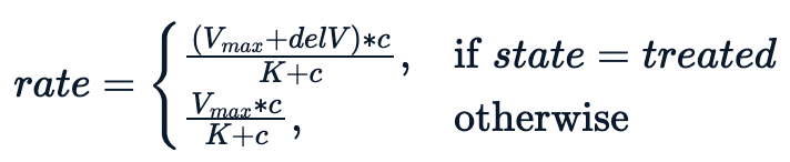
One can visualize how the tuned model performs by plotting a fitted line on the data, no surprise, the tuned model gives us a better fit for different classes.

plot(Puromycin$conc, Puromycin$rate, xlab="conc", ylab = "rate")
lines(Puromycin[Puromycin$state == "treated",]$conc, predict(Purboth, Puromycin[Puromycin$state == "treated",]), col=2)
lines(Puromycin[Puromycin$state != "treated",]$conc, predict(Purboth, Puromycin[Puromycin$state != "treated",]), col=3)
legend(0, 200, legend = c("treated", "untreated"), fill = c(2,3))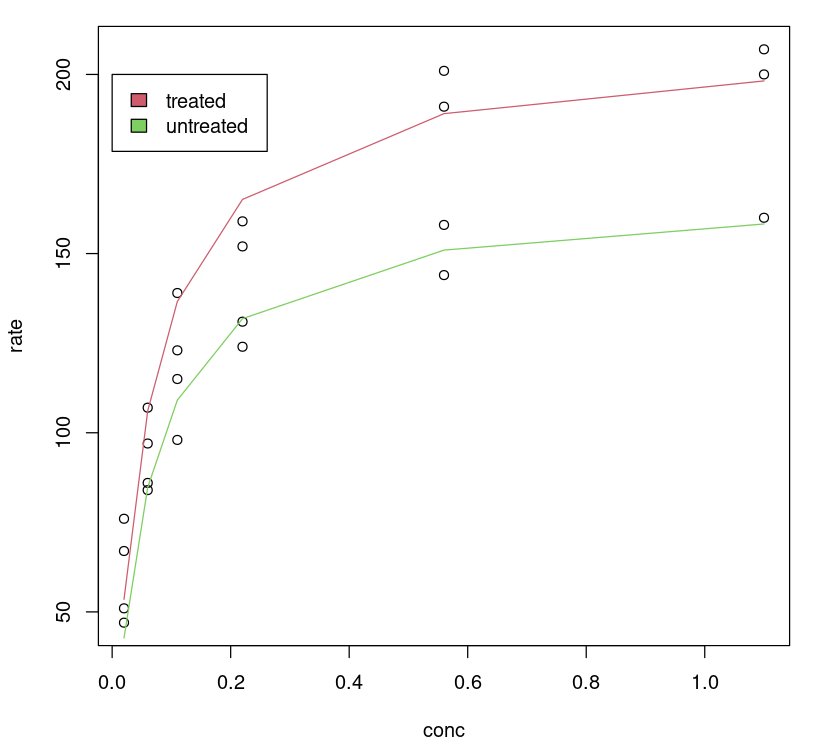

Confidence Interval of Parameters

One cannot rely on p-values, the 95% confidence interval gives the coefficient values for each significant parameter at 2.5% and 97.5%. None of them include 0.

confint(Purboth)

Using the confidence interval value, one can statistically say that there is a 95 % chance that a true value of the parameter e.g Vmax falls within the range given above, which is (154.62, 179.25) for Vmax.

Profiling

One can further profile the model to understand the uncertainty in parameter estimation by examining the objective function directly. In our model, we have three parameters, Vmax,delV, K we can profile them:

• To get the confidence interval.
• And use the profile function t, which is similar to the t-statistics used by the linear model. Plots of the profile t function provides the likelihood intervals for individual parameters and explains how non-linear the estimation is.

Plotting the confidence interval

This plots the confidence interval of parameters for different values of (which corresponds to different confidence intervals (99%, 95%, 90%, 80% and 50%). It is similar to the confidence interval (95%) provided by confint(object, parm, level = 0.95, ...)function.

Purbothpf = profile(Purboth)
par( mfrow= c(2,2) )
plot(Purbothpf)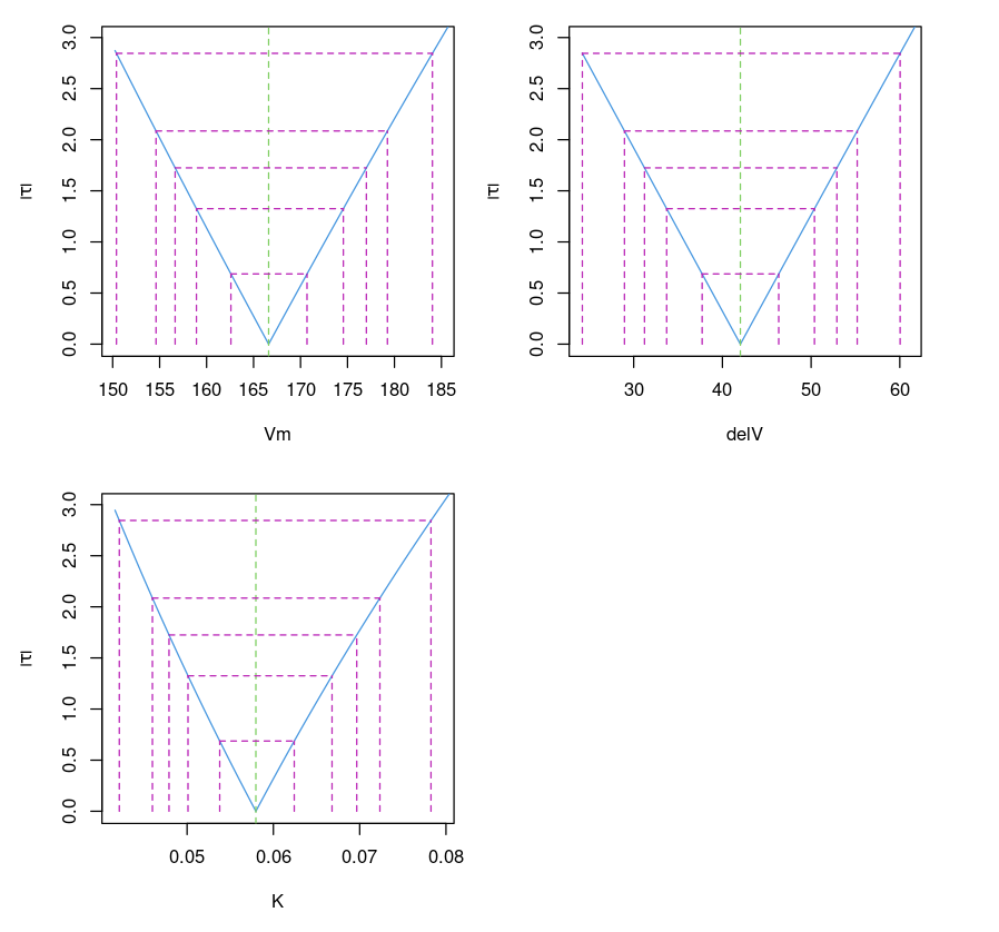

Plotting _T vs parameters

Plotting three parameters Vmax,delV, K vs _T gives us a feeling if the fit is linear or non-linear. One can observe that the line appears linear for parameters delV and Vm, and slightly curved for K. This is expected because the parameter K exhibits a non-linear relation.

dataVm = data.frame(Purbothpf$Vm$par.vals)
datadelV = data.frame(Purbothpf$delV$par.vals)
dataK = data.frame(Purbothpf$K$par.vals)
par( mfrow= c(2,2) )
plot(dataVm$Vm,Purbothpf$Vm$tau, type="l", xlab = "Vm", ylab = "Tau")
plot(datadelV$delV,Purbothpf$delV$tau, type="l", xlab = "delV", ylab = "Tau")
plot(dataK$K,Purbothpf$K$tau, type="l", xlab = "K", ylab = "Tau")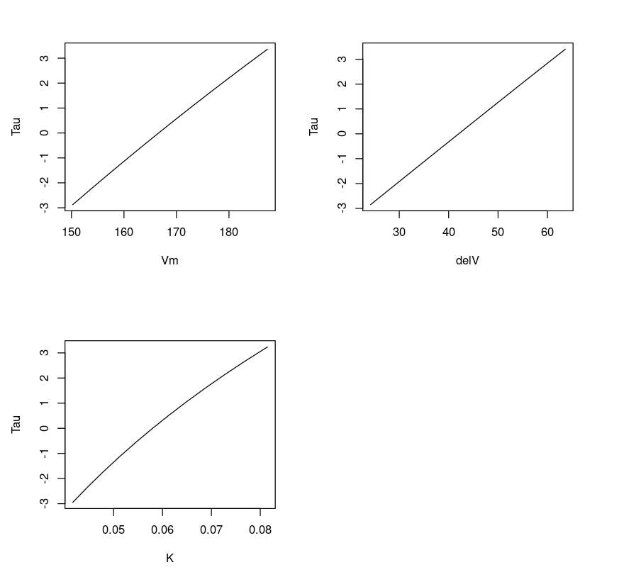

Fitting a Linear Model

One can use the same R library function nls() to fit in a linear model as shown below. I feel it is a good habit to always try a linear model for interpretability and comparison.

PurbothRealLinear <- nls(rate ~ i + m*conc, Puromycin, list(i=160, m=0.05) )
summary(PurbothRealLinear)

Formula: rate ~ i + m * conc

Parameters:
  Estimate Std. Error t value Pr(>|t|)    
i    93.92       8.00   11.74 1.09e-10 ***
m   105.40      16.92    6.23 3.53e-06 ***
---
Signif. codes:  0 ‘***’ 0.001 ‘**’ 0.01 ‘*’ 0.05 ‘.’ 0.1 ‘ ’ 1

Residual standard error: 28.82 on 21 degrees of freedom

Number of iterations to convergence: 2 
Achieved convergence tolerance: 2.571e-09

Although the parameters look significant, it is a poor fit. The residual standard error is high.

Visualizing the Fit

It seems the linear model performs poorly; one can visualize it by plotting a fitted line on the data and comparing it with its non-linear counterpart.

plot(Puromycin$conc, Puromycin$rate, xlab="conc", ylab = "rate")
lines(Puromycin$conc, predict(PurbothRealLinear), col=4)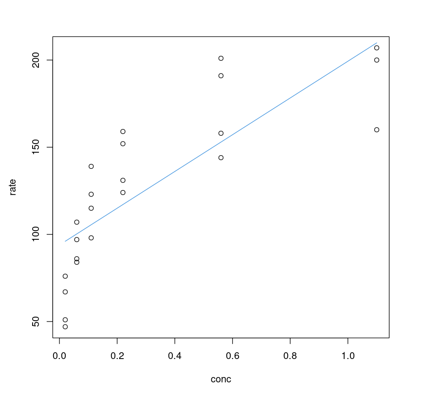

Compare Non Linear vs Linear Model Analytically

From the above plot, we know the linear model does a poor job, but how do we compare these models? It will be like comparing apples to oranges. AIC results cannot be directly used.

Goodness of Fit

What constitutes a good fit - for regression, it is the predicted and the actual value being as close as possible. So if we inspect the quality of what a model has predicted using a R lm() function one can compare them. The model that is more accurate will have the points fall close to the ideal line. An ideal line is a model that is 100 % accurate - the predicted is the same as the actual value for each data point. Therefore, all the points will be on a straight line.

Non-Linear Fit

So for each input data point, we use the model to predict the target value and then apply the lm() function as shown. By plotting a scatter plot between the actual rate (x-axis) and the predicted rate (y-axis) and drawing an ideal line, one can observe how close the points are to the line.

nonLinear_df = data.frame("rate"=Puromycin$rate, "pred_rate"= predict(Purboth))
fit_nonLinear = lm(nonLinear_df$rate ~ nonLinear_df$pred_rate)
AIC(fit_nonLinear)
plot(nonLinear_df$rate, nonLinear_df$pred_rate, xlab="actual_rate", 
     ylab = "pred_rate", 
     main = "Comparing Actual vs Predicted for Non Linear Model")
lines(Puromycin$rate, Puromycin$rate)

174.711198508104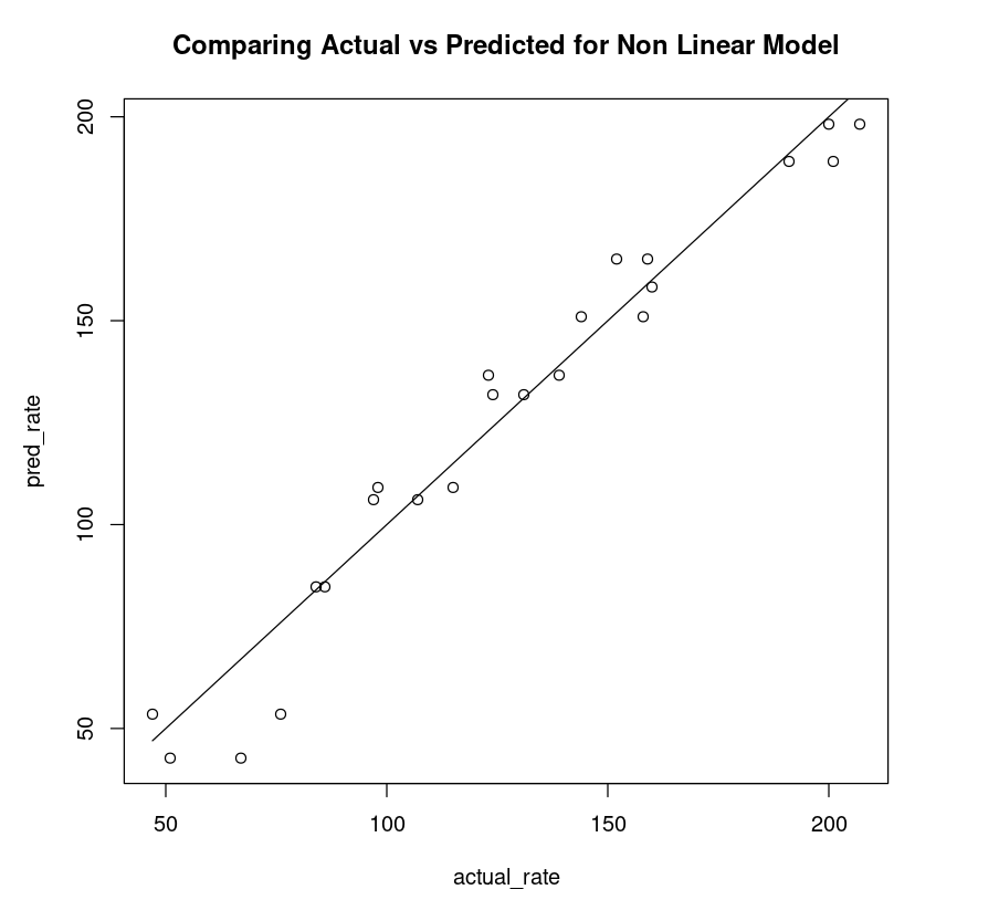

Linear Fit

The non-linear plot above is clearly a better fit compared to the linear plot (below).

linear_df = data.frame("rate"=Puromycin$rate, "pred_rate"= predict(PurbothRealLinear))
fit_linear = lm(linear_df$rate~linear_df$pred_rate)
AIC(fit_linear)
plot(linear_df$rate, linear_df$pred_rate, xlab="actual_rate", ylab = "pred_rate", 
     main= "Comparing Actual vs Predicted using lm()")
lines(Puromycin$rate, Puromycin$rate)

223.783416979551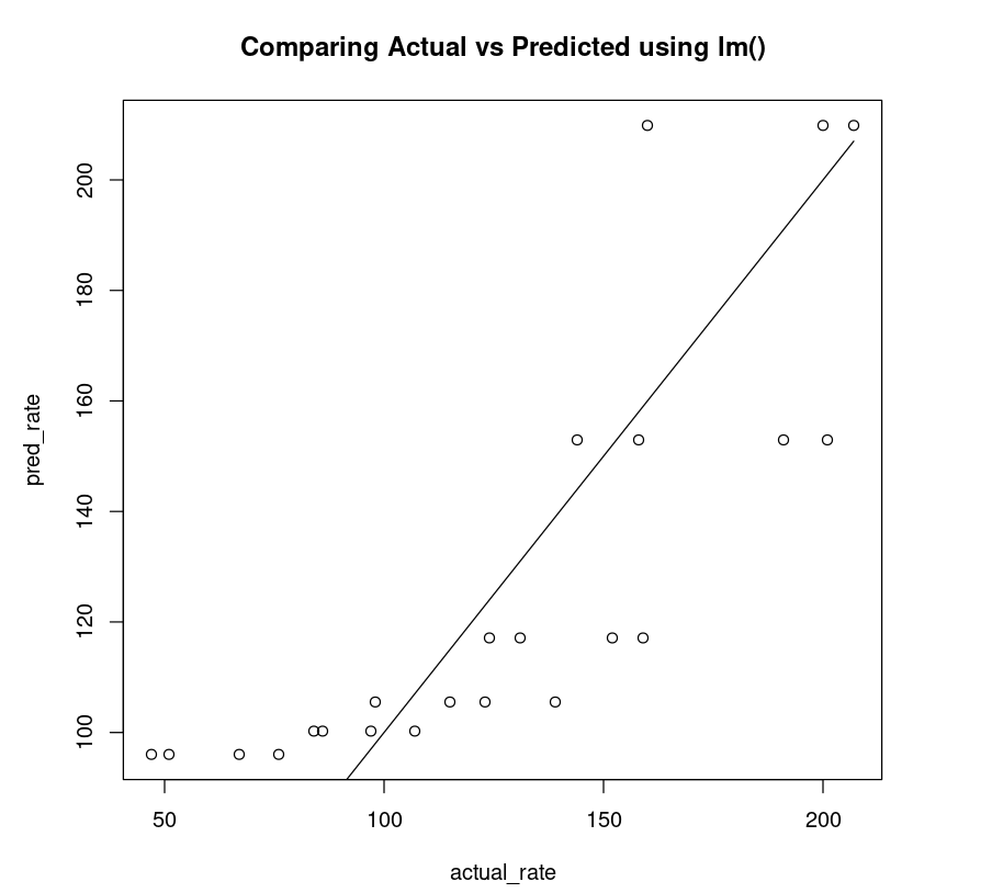

Improving Linear Model

It seems we are unfair to the linear model because we clearly see the data do not follow a straight line so we can try to fit the model using transformed data. We choose sqrt() to transform the conc and fit a linear model as shown below.

PurbothLinearSqrt = nls(rate ~ i + m*sqrt(conc), Puromycin, list(i=160, m=0.05) )
summary(PurbothLinearSqrt)

Formula: rate ~ i + m * sqrt(conc)

Parameters:
  Estimate Std. Error t value Pr(>|t|)    
i   60.961      8.758   6.961 7.11e-07 ***
m  139.134     15.675   8.876 1.50e-08 ***
---
Signif. codes:  0 ‘***’ 0.001 ‘**’ 0.01 ‘*’ 0.05 ‘.’ 0.1 ‘ ’ 1

Residual standard error: 22.31 on 21 degrees of freedom

Number of iterations to convergence: 2 
Achieved convergence tolerance: 1.838e-09

Indeed, there is a drop in residual standard error, but it is less than what we were expecting.

Plotting the fit

One can definitely see that using sqrt() on conc improves the linear model. However, compared to the non-linear model Purboth it is not any better. The residual standard error of PurbothLinearSqrt model is almost double of Purboth therefore we won't analyze this model any further. One can try to fit higher-order polynomial terms (using polynomial regression) but the effort required to fine-tune that model is a lot more when one can achieve better results using a non-linear model.

plot(Puromycin$conc, Puromycin$rate, xlab="conc", ylab = "rate")
lines(Puromycin[Puromycin$state != "treated",]$conc, predict(PurbothLinearSqrt, Puromycin[Puromycin$state != "treated",]), col=2)
lines(Puromycin[Puromycin$state != "treated",]$conc, predict(PurbothLinearSqrt, Puromycin[Puromycin$state != "treated",]), col=3)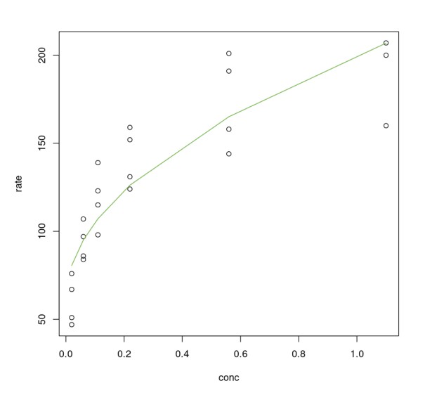

Unwinding the Non-Linearity Equation

One can apply a trick to unwind a non-linear function and fit a linear model. This technique was used in the past when the calculations were done by hand, not by computers. However, such models fail to do a better job.

Converting Non-Linear to Linear Form

As an illustration, one can change the Michaelis-Menten equation by taking its inverse, as shown below, and use the modified form to apply a linear model.

We can use the same nls() to fit the new equation.

PurbothPseudoLinear <- nls((1/rate) ~ K /(Vm*conc) + 1/Vm , Puromycin, 
                           list(Vm=160, K=0.05))
summary(PurbothPseudoLinear)

Formula: (1/rate) ~ K/(Vm * conc) + 1/Vm

Parameters:
    Estimate Std. Error t value Pr(>|t|)    
Vm 1.674e+02  1.362e+01  12.287 4.70e-11 ***
K  3.900e-02  6.172e-03   6.318 2.89e-06 ***
---
Signif. codes:  0 ‘***’ 0.001 ‘**’ 0.01 ‘*’ 0.05 ‘.’ 0.1 ‘ ’ 1

Residual standard error: 0.001786 on 21 degrees of freedom

Number of iterations to convergence: 3 
Achieved convergence tolerance: 2.997e-09

The residual standard error is low, but the data used, therefore, cannot be used to compare with non-linear models. Our best bet is to visualize how both models perform on the original dataset.

Plotting the fit

We compare Purboth_1 model, which uses two parameters Vmax, K with PurbothPseudoLinear.The plot clearly shows a non-linear model does a better job.

plot(Puromycin$conc, Puromycin$rate, xlab="conc", ylab = "rate", 
     main = "Scatterplot conc vs rate")
lines(Puromycin[Puromycin$state == "treated",]$conc, 
      predict(Purboth_1, Puromycin[Puromycin$state == "treated",]), col=2)
lines(Puromycin[Puromycin$state != "treated",]$conc, 
      predict(Purboth_1, Puromycin[Puromycin$state != "treated",]), col=2)
lines(Puromycin[Puromycin$state == "treated",]$conc, 
      1/predict(PurbothPseudoLinear, Puromycin[Puromycin$state == "treated",])
      , col=4)
lines(Puromycin[Puromycin$state != "treated",]$conc, 
      1/predict(PurbothPseudoLinear, Puromycin[Puromycin$state != "treated",])
      , col=4)
legend(0, 200, legend = c("nls", "nls-turned-linear"), fill = c(2,4))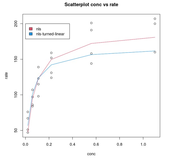

Goodness of Fit

One can compare the goodness of the model.

nonLinear_df = data.frame("rate"=Puromycin$rate, "pred_rate"= predict(Purboth_1))
fit_nonLinear = lm(nonLinear_df$rate ~ nonLinear_df$pred_rate)
AIC(fit_nonLinear)

203.017860461858

linear_df = data.frame("rate"=Puromycin$rate, 
                       "pred_rate"= 1/predict(PurbothPseudoLinear))
fit_linear = lm(linear_df$rate~linear_df$pred_rate)
AIC(fit_linear)

206.999538212925

This shows a model that uses a non-linear function performs much better.

par( mfrow= c(1,2) )
plot(nonLinear_df$rate, nonLinear_df$pred_rate, xlab="actual_rate", 
     ylab = "pred_rate", 
     main = "Non-Linear")
lines(Puromycin$rate, Puromycin$rate)

plot(linear_df$rate, linear_df$pred_rate, xlab="actual_rate", ylab = "pred_rate", 
     main = "Turned Linear")
lines(Puromycin$rate, Puromycin$rate)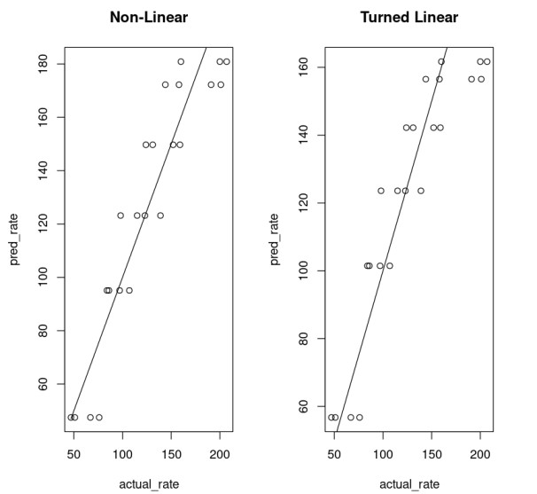

Conclusion

The non-linear model performs better than the linear counterpart, especially in cases where we have mechanistic data. However, a non-linear model does not guarantee a numerical solution to an estimation problem. One can plot and select a mathematical function that may best explain the relationship between data. In such cases, the non-linear model may supersede its linear counterpart.

If you found this article enlightening and want to dive deeper into the world of regression models, check out DataCamp's Intermediate Regression in R course.