Loss Functions in Machine Learning Explained

Machine learning provides computational models with the capability to make predictions, classifications, and decisions based on data. As a field of study, machine learning is a subset of the domain of artificial intelligence, which encapsulates the processes involved in building a computational model with capabilities that mimic human intelligence and, in some cases, surpass it.

Machine learning and associated algorithms and techniques fundamentally involve designing, implementing, and training algorithms to recognize patterns in exposed data and perform predictions or classifications.

Machine learning algorithms learn through different methods, but a fundamental component of the learning process of machine learning algorithms and models is the loss function. The loss function is a mathematical process that quantifies the error margin between a model's prediction and the actual target value. Later in this article, we explore the loss function in detail.

Loss Functions in Brief

The key takeaway is that the loss function is a measurable way to gauge the performance and accuracy of a machine learning model. In this case, the loss function acts as a guide for the learning process within a model or machine learning algorithm.

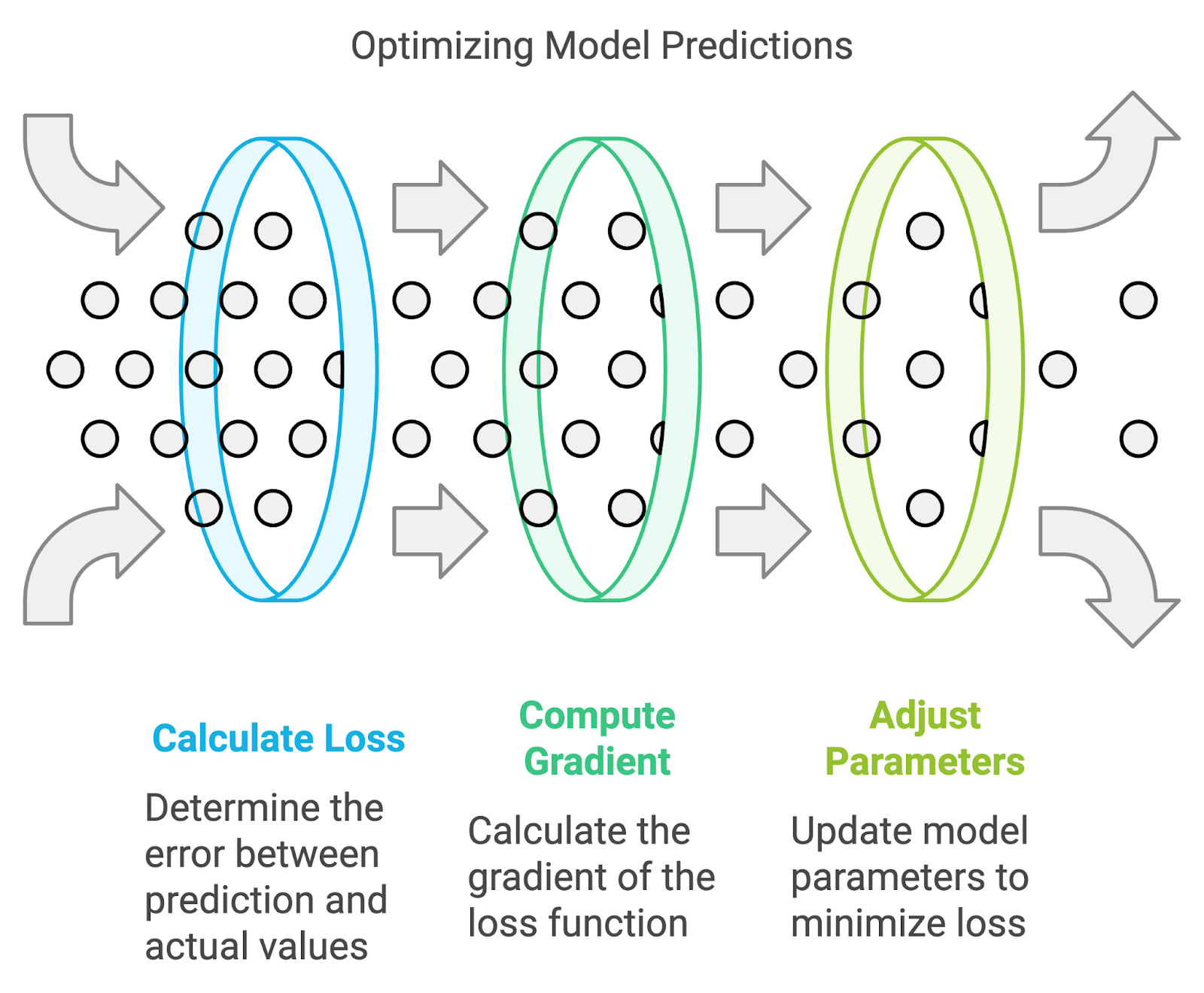
The role of the loss function is crucial in the training of machine learning models and includes the following:

• Performance measurement: Loss functions offer a clear metric to evaluate a model's performance by quantifying the difference between predictions and actual results.
• Direction for improvement: Loss functions guide model improvement by directing the algorithm to adjust parameters(weights) iteratively to reduce loss and improve predictions.
• Balancing bias and variance: Effective loss functions help balance model bias (oversimplification) and variance (overfitting), essential for the model's generalization to new data.
• Influencing model behavior: Certain loss functions can affect the model's behavior, such as being more robust against data outliers or prioritizing specific types of errors.

Let's explore the roles of particular loss functions in later sections and build a detailed intuition and understanding of the loss function.

What is a Loss Function?

The loss function, also referred to as the error function, is a crucial component in machine learning that quantifies the difference between the predicted outputs of a machine learning algorithm and the actual target values. For example, within a regression problem to predict car prices based on historical data, a loss function evaluates a neural network prediction based on a training sample from the training dataset. The loss function quantifies the gap or the error margin of the car price predicted by the network to the actual price.

The resulting value, the loss, reflects the accuracy of the model's predictions. During training, a learning algorithm such as the backpropagation algorithm uses the gradient of the loss function with respect to the model's parameters to adjust these parameters and minimize the loss, effectively improving the model's performance on the dataset.

Often, the terms loss function and cost function are used interchangeably; despite this, both terms have distinct definitions:

As mentioned earlier, the loss function, also known as the error function, quantifies how well a single prediction of the machine learning algorithm is compared to the actual target value. The key takeaway is that a loss function applies to a single training example and is part of the overall model's learning process that provides the signal by which the model's learning algorithm updates the weights and parameters.

The cost function, sometimes called the objective function, is an average of the loss function of an entire training set containing several training examples. The cost function quantifies the model's performance on the whole training dataset.

Let’s delve deeper into how loss functions work.

How Loss Functions Work

Although there are different types of loss functions, fundamentally, they all operate by quantifying the difference between a mode’s predictions and the actual target value in the dataset. The official term for this numerical quantification is the prediction error. The learning algorithm and mechanisms in a machine learning model are optimized to minimize the prediction error, so this means that after a calculation of the value for the loss function, which is determined by the prediction error, the learning algorithm leverages this information to conduct weight and parameter updates which in effect during the next training pass leads to a lower prediction error.

When exploring the topic of loss function, machine learning algorithms, and the learning process within neural networks, the topic of Empirical Risk Minimization(ERM) comes up. ERM is an approach to selecting the optimal parameters of a machine learning algorithm that minimizes the empirical risk. The empirical risk, in this case, is the training dataset.

The risk minimization component of ERM is the process by which the internal learning algorithm minimizes the error of prediction of machine learning algorithm to a known dataset in the outcome that the model has an expected performance and accuracy in a scenario where an unseen dataset or data sample which could have similar statical data distribution as the dataset the model’s has been initially trained on.

Types of Loss Functions

Loss functions in machine learning can be categorized based on the machine learning tasks to which they are applicable. Most loss functions apply to regression and classification machine learning problems. The model is expected to predict continuous output values for regression machine learning tasks. In contrast, the model is expected to provide discrete labels corresponding to a dataset class for classification tasks.

Below are standard loss functions and their classification into machine learning problems they lend themselves well to. Most of these loss functions are covered in detail later in this article.

Loss Functions for Regression

Mean Square Error (MSE) / L2 Loss

The Mean Square Error(MSE) or L2 loss is a loss function that quantifies the magnitude of the error between a machine learning algorithm prediction and an actual output by taking the average of the squared difference between the predictions and the target values. Squaring the difference between the predictions and actual target values results in a higher penalty assigned to more significant deviations from the target value. A mean of the errors normalizes the total errors against the number of samples in a dataset or observation.

The mathematical equation for Mean Square Error (MSE) or L2 Loss is:

MSE = (1/n) * Σ(yᵢ - ȳ)²

Where:

• n is the number of samples in the dataset
• yᵢ is the predicted value for the i-th sample
• ȳ is the target value for the i-th sample

When to use MSE

Understanding when to use MSE is crucial in machine learning model development. MSE is a standard loss function utilized in most regression tasks since it directs the model to optimize to minimize the squared differences between the predicted and target values.

MSE is recommended for ML scenarios where it is conducive to the learning process to penalize significantly the presence of outliers. However, these characteristics of MSE are not always suitable for scenarios and use cases where outliers are due to noise from the data as opposed to positive signals.

An example scenario of when the MSE loss function is leveraged is in real estate price prediction or, more broadly, predictive modelling. Predicting house prices involves using features such as the number of rooms, location, area, distance from amenities and other numerical features. House prices in a localized area are normally distributed, so the objective to penalize outliers is essential to the model’s ability to predict accurate house prices.

A small percentage error in real estate can equate to a significant amount of money. For instance, a 5% error in a $200,000 house is $10,000, which is substantial. Hence, squaring the errors (as done in MSE) helps in giving higher weight to larger errors, thus pushing the model to be more precise with higher-valued properties.

Mean Absolute Error (MAE) / L1 Loss

Mean Absolute Error (MAE), also known as L1 Loss, is a loss function used in regression tasks that calculates the average absolute differences between predicted values from a machine learning model and the actual target values. Unlike Mean Squared Error (MSE), MAE does not square the differences, treating all errors with equal weight regardless of their magnitude.

The mathematical equation for Mean Absolute Error (MAE) or L1 Loss is:

MAE = (1/n) * Σ|yᵢ - ȳ|

Where:

• n is the number of samples in the dataset
• yᵢ is the predicted value for the i-th sample
• ȳ is the target value for the i-th sample

When to use MAE

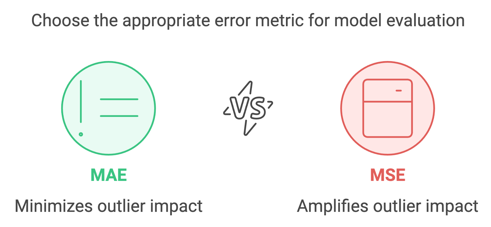
MAE measures the average absolute difference between the predicted and actual values. Unlike MSE, MAE does not square the differences, which makes it less sensitive to outliers. Compared to Mean Squared Error (MSE), Mean Absolute Error (MAE) is inherently less sensitive to outliers because it assigns an equal weight to all errors, regardless of their magnitude.

This means that while an outlier can significantly skew the MSE by contributing a disproportionately large error when squared, its impact on MAE is much more contained. An outlier's influence on the overall error metric is minimal when using MAE as a loss function. In contrast, MSE amplifies the effect of outliers due to the squaring of error terms, affecting the model's error estimation more substantially.

A scenario where MAE is an applicable loss function is one where we don't want to penalize outliers considerably or at all, for example, predicting delivery times for a food delivery company.

A delivery services company such as UberEats, Deliveroo, or DoorDash might build a delivery estimation model to increase customer satisfaction. The time taken for a delivery service to get food delivered is affected by several factors such as weather, traffic incidents, roadworks, etc.

Handling these factors is crucial to the estimation of delivery times. One method of handling this is to classify these events as outliers but make the decision to ensure it doesn't affect the model being trained. MAE is a suitable loss function within this scenario as it will treat data points that are outliers due to roadworks or rare events with less severity, reducing the effect of the outliers on the error metric and model's learning process.

MAE notably adds a uniform error weighting to all data points; in the scenario described, penalizing outlier data points could result in over-estimating or under-estimating delivery times.

Huber Loss / Smooth Mean Absolute Error

Huber Loss or Smooth Mean Absolute Error is a loss function that takes the advantageous characteristics of the Mean Absolute Error and Mean Squared Error loss functions and combines them into a single loss function. The hybrid nature of Huber Loss makes it less sensitive to outliers, just like MAE, but also penalizes minor errors within the data sample, similar to MSE. The Huber Loss function is also utilized in regression machine learning tasks.

The mathematical equation for Huber Loss is as follows:

L(δ, y, f(x)) = (1/2) * (f(x) - y)^2   if |f(x) - y| <= δ
               = δ * |f(x) - y| - (1/2) * δ^2   if |f(x) - y| > δ

Where:

• L represents the Huber Loss function
• δ is the delta parameter, which determines the threshold for switching between the quadratic and linear components of the loss function
• y is the true value or target value
• f(x) is the predicted value

When to use Huber Loss / Smooth Mean Absolute Error

The Huber Loss function effectively combines two components for handling errors differently, with the transition point between these components determined by the threshold δ:

• Quadratic Component for Small Errors: For errors smaller than δ, it uses the quadratic component (1/2) * (f(x) - y)^2
• Linear Component for Large Errors: For errors larger than δ, it applies the linear component δ * |f(x) - y| - (1/2) * δ^2

Huber loss operates in two modes that are switched based on the size of the calculated difference between the actual target value and the prediction of the machine learning algorithm. The key term within Huber Loss is delta (δ). Delta is a threshold that determines the numerical boundary at which the Huber Loss utilizes the quadratic application of loss or linear calculation.

The quadratic component of Huber Loss characterizes the advantages of MSE that penalize outliers; within Huber Loss, this is applied to errors smaller than delta, which ensures a more accurate prediction from the model.

Suppose the calculated error, which is the difference between the actual and predicted values, is larger than the delta. In that case, Huber Loss utilizes the linear calculation of loss similar to MAE, where there is less sensitivity to the error size to ensure the trained model isn’t over-penalizing large errors, especially if the dataset contains outliers or unlikely-to-occur data samples.

Loss Functions for Classification

Binary Cross-Entropy Loss / Log Loss

Binary Cross-Entropy Loss(BCE) is a performance measure for classification models that outputs a prediction with a probability value typically between 0 and 1, and this prediction value corresponds to the likelihood of a data sample belonging to a class or category. In the case of Binary Cross-Entropy Loss, there are two distinct classes. But notably, a variant of cross-entropy loss, Categorical Cross-Entropy applies to multiclass classification scenarios.

To understand Binary Cross-Entropy Loss, sometimes called Log Loss, it is helpful to discuss the components of the terms.

• Loss: This is a mathematical quantification of the margin/difference between the prediction of a machine learning algorithm and the actual target value.
• Entropy: A simple definition of entropy is that it is a calculation of the degree of randomness or disorder within a system
• Cross Entropy: This is a term commonly utilised in information theory, and it measures the differences between two probability distributions that can be used to identify an observation.
• Binary: This is an expression of numerical digits using either of two states, 0 or 1. This is extended to the definition of Binary Classification where we ditingus=ish two classes(A and B) using binary representation, where class A is assigned the numerical representation of 0 and class B is assigned 1.

Binary Cross Entropy Loss (or Log Loss) is a quantification of the difference between the prediction of a machine learning algorithm and the actual target prediction that is calculated from the negative value of the summation of the logarithm value of the probabilities of the predictions made by the machine learning algorithm against the total number of data samples. BCE is found in machine learning use cases that are logistic regression problems and in training artificial neural networks designed to predict the likelihood of a data sample belonging to a class and leverage the sigmoid activation function internally.

The mathematical equation for Binary Cross-Entropy Loss, also known as Log Loss, is:

L(y, f(x)) = -[y * log(f(x)) + (1 - y) * log(1 - f(x))]

Where:

• L represents the Binary Cross-Entropy Loss function
• y is the true binary label (0 or 1)
• f(x) is the predicted probability of the positive class (between 0 and 1)

When to use Binary Cross-Entropy Loss / Log Loss

The equation above specifically applies to a scenario where the machine learning algorithm will make a classification between two classes. This is a binary classification scenario.

As noted in the equation by the negative symbol: ‘-’ BCE calculates the loss by determining the negative of two terms, and for several predictions or data samples, the average of the negative of the following two terms:

1. The logarithm of the model’s predicted probability went the positive class is present y * log(f(x))
2. The logarithm of 1 minus the predicted probability of the negative class: (1 - y) * log(1 - f(x))

The BCE loss function penalizes inaccurate predictions, which are predictions that have a significant difference from the positive class or, in other words, have a high quantification of entropy. When BCE is utilized as a component within learning algorithms, this encourages the model to refine its predictions, which are probabilities for the appropriate class during its training.

Hinge Loss

Hinge Loss is a loss function utilized within machine learning to train classifiers that optimize to increase the margin between data points and the decision boundary. Hence, it is mainly used for maximum margin classifications. To ensure the maximum margin between the data points and boundaries, hinge loss penalizes predictions from the machine learning model that are wrongly classified, which are predictions that fall on the wrong side of the margin boundary and also predictions that are correctly classified but are within close proximity to the decision boundary.

This characteristic of the Hinge Loss function ensures machine learning models are able to predict the accurate classification of data points to their target value with confidence that exceeds the threshold of the decision boundary. This approach to machine algorithm learning enhances the model's generalization capabilities, making it effective for accurately classifying data points with a high degree of certainty.

The mathematical equation for Hinge Loss is:

L(y, f(x)) = max(0, 1 - y * f(x))

Where:

• L represents the Hinge Loss
• y is the true label or target value (-1 or 1)
• f(x) is the predicted value or decision function output

Choosing the Right Loss Function

Selecting the appropriate loss function to apply to a machine learning algorithm is essential, as the model's performance heavily depends on the algorithm's ability to learn or adapt its internal weights to fit a dataset.

A machine learning model or algorithm's performance is defined by the loss function utilized, mainly because the loss function component affects the learning algorithm used to minimize the model's error loss or cost function value. Essentially, the loss function impacts the model's ability to learn and adapt the value of its internal weights to fit the patterns within a dataset.

When appropriately selected, the loss function enables the learning algorithm to effectively converge to an optimal loss during its training phase and generalize well to unseen data samples. An appropriately selected loss function acts as a guide, steering the learning algorithm towards accuracy and reliability, ensuring that it captures the underlying patterns in the data while avoiding overfitting or underfitting.

Factors to consider when selecting a loss function

Understanding the type of machine learning problem at hand helps determine a category of loss function to utilize. Different loss functions apply to various machine-learning problems.

Classification vs Regression

Classification machine learning tasks usually involve assigning data points to a specific category label. With this type of machine learning task, the output of the machine learning model is typically a set of probabilities that determine the likelihood of a data point being a certain label.

The cross-entropy loss function is commonly used for classification tasks. In a machine learning regression task where the objective is for a machine learning model to produce a prediction based on a set of inputs, loss functions such as mean squared error or mean absolute error are better suited.

Binary vs Multiclass Classification

Binary classification involves the categorization of data samples into two distinct categories, whereas multiclass classification, as the name suggests, involves the categorization of data samples into more than two categories. For machine learning classification problems that involve just two classes(binary classification), leveraging a binary cross-entropy loss function is best. In situations where more than two classes are targets for predictions, categorical cross-entropy should be utilized.

Sensitivity

Another factor to consider is the sensitivity of the loss function to outliers. In some scenarios, it is desirable to ensure that outliers and data samples that skew the overall statistical distribution of the dataset are penalized during training; in such scenarios, loss functions such as mean squared error are suitable.

Whereas there are scenarios where less sensitivity to outliers is required, these are scenarios where outliers could be 'never events' or unlikely to happen. For this objective, penalizing outliers might produce a non-performant model. Loss function such as mean absolute error is applicable in such scenarios. For the best of both worlds, practitioners should consider the Huber loss function, which takes components that penalize outliers with low error values and reduce the model's sensitivity to outliers with large error values.

Computational efficiency

Computational resource is a commodity within machine learning, commercial, and research domain. Access to large computing capacity enables practitioners the flexibility to experiment with large datasets and solve more complex machine-learning problems. Some loss functions are more computationally demanding than others, especially when the number of datasets is large. This makes the computational efficiency of a loss function a factor to consider during the selection process of a loss function.

Impact of outliers and data distribution

Outliers are data samples that fall outside the overall statistical distribution of a dataset; they are sometimes referred to as anomalies or irregularities. How outliers are managed determines the performance and accuracy of the trained machine learning model.

As mentioned earlier, outliers in datasets affect the error values utilized in loss functions, depending on the loss function used. The effect of outliers on the loss functions propagates to the outcome of the learning process of the machine learning algorithm, which can lead to intended or unintended behavior from the machine learning algorithm or model.

For example, mean squared error penalizes outliers contributing to large error values/terms; this means during the training process, the model weights are adjusted to learn how to accommodate these outliers. Again, if this isn’t the intended behavior of the machine learning model, the finalized model created after training will have poor generalization to unseen data. For scenarios where mitigating the impact of outliers is required, functions such as MAE and Huber loss are more applicable.

Implementing Loss Functions

Examples of implementing common loss functions

Implementation of MAE in Python

# Python implementation of Mean Absolute Error (MAE)

def mean_absolute_error(actual:list, predicted:list) -> float:
    """
    Calculate the Mean Absolute Error between actual and predicted values

    :param actual: list, actual values
    :param predicted: list, predicted values
    :return: float, the calculated MAE
    """
    # Ensure the length of the two lists are the same
    if len(actual) != len(predicted):
        raise ValueError("The length of actual values and predicted values must be the same")

    # Calculate the absolute differences
    absolute_diffs = [abs(act - pred) for act, pred in zip(actual, predicted)]
    
    # Calculate the mean of the absolute differences
    mae = sum(absolute_diffs) / len(actual)
    
    return mae

# Example usage:
# actual values
y_true = [3, -0.5, 2, 7]

# predicted values
y_pred = [2.5, 0.0, 2, 8]

# Calculate MAE
mae_value = mean_absolute_error(y_true, y_pred)
print(mae_value)
# 0.5

Implementation of MSE in Python

# Python implementation of Mean Squared Error (MSE) / L2 Loss

def mean_squared_error(actual:list, predicted:list) -> float:
    """
    Calculate the Mean Squared Error between actual and predicted values

    :param actual: list, actual values
    :param predicted: list ,predicted values
    :return: float, the calculated MSE
    """
    # Ensure the length of the two lists are the same
    if len(actual) != len(predicted):
        raise ValueError("The length of actual values and predicted values must be the same")

    # Calculate the squared differences
		# (yᵢ - ȳ)²
    squared_diffs = [(act - pred) ** 2 for act, pred in zip(actual, predicted)]
    
    # Calculate the mean of the squared differences
    mse = sum(squared_diffs) / len(actual)
    
    return mse

# Example usage:
# actual values
y_true = [1, 2, 3, 4, 5]

# predicted values
y_pred = [1.1, 2.2, 2.9, 4.1, 4.9]

# Calculate MSE
mse_value = mean_squared_error(y_true, y_pred)
print(mse_value)
# 0.015999999999999993

The use of libraries for loss function implementation

While custom implementation of loss functions is feasible, and deep learning libraries like TensorFlow and PyTorch support the use of bespoke loss functions in neural network implementations, libraries such as Scikit-learn, TensorFlow, and PyTorch offer built-in implementations of commonly used loss functions.

These pre-integrated functionalities facilitate easy leverage and abstract away the complexities involved in implementing these loss functions, streamlining the development process for machine learning models.

Utilizing these deep learning libraries provides advantages over pure Python implementations, some of which are:

• Ease of use
• Efficiency and optimisation
• GPU and parallel computing support
• Developer community support

Mean Absolute Error (MAE) using the scikit-learn library

from sklearn.metrics import mean_absolute_error

# actual values
y_true = [3, -0.5, 2, 7]

# predicted values
y_pred = [2.5, 0.0, 2, 8]

# Calculate MAE using scikit-learn
mae_value = mean_absolute_error(y_true, y_pred)
print(mae_value)
#0.5

Mean Squared Error (MSE) using the scikit-learn library

from sklearn.metrics import mean_squared_error

# actual values
y_true = [1, 2, 3, 4, 5]

# predicted values
y_pred = [1.1, 2.2, 2.9, 4.1, 4.9]

# Calculate MSE using scikit-learn
mse_value = mean_squared_error(y_true, y_pred)
print(mse_value)
# 0.016

Conclusion

In summary, choosing the right loss function is crucial for effective machine learning model training. This article highlighted key loss functions, their roles in machine learning algorithms, and their suitability for different tasks. From Mean Squared Error (MSE) to Huber Loss, each function has its unique advantages, whether it's handling outliers or balancing bias and variance.

The decision to use custom or pre-built loss functions from libraries like Scikit-learn, TensorFlow, and PyTorch hinges on specific project needs, computational efficiency, and user expertise. These libraries offer ease of implementation, ongoing community support, and regular updates.

Despite the evolution of machine learning, the importance of loss functions remains constant. Future trends may bring more specialized loss functions, but the fundamental principles will likely persist. For a deeper dive into machine learning and its applications, explore DataCamp’s Machine Learning Scientist with Python track.