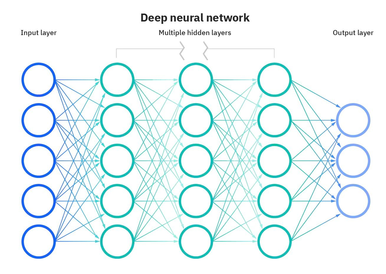
Representation of Neural Network. Image Source
What Are Activation Functions?
Activation functions are an integral building block of neural networks that enable them to learn complex patterns in data. They transform the input signal of a node in a neural network into an output signal that is then passed on to the next layer. Without activation functions, neural networks would be restricted to modeling only linear relationships between inputs and outputs.
Activation functions introduce non-linearities, allowing neural networks to learn highly complex mappings between inputs and outputs.
Choosing the right activation function is crucial for training neural networks that generalize well and provide accurate predictions. In this post, we will provide an overview of the most common activation functions, their roles, and how to select suitable activation functions for different use cases.
Whether you are just starting out in deep learning or are a seasoned practitioner, understanding activation functions in depth will build your intuition and improve your application of neural networks.
Why Are Activation Functions Essential?
Without activation functions, neural networks would just consist of linear operations like matrix multiplication. All layers would perform linear transformations of the input, and no non-linearities would be introduced.
Most real-world data is non-linear. For example, relationships between house prices and size, income, and purchases, etc., are non-linear. If neural networks had no activation functions, they would fail to learn the complex non-linear patterns that exist in real-world data.
Activation functions enable neural networks to learn these non-linear relationships by introducing non-linear behaviors through activation functions. This greatly increases the flexibility and power of neural networks to model complex and nuanced data.
Types of Activation Functions
Neural networks leverage various types of activation functions to introduce non-linearities and enable learning complex patterns. Each activation function has its own unique properties and is suitable for certain use cases.
For example, the sigmoid function is ideal for binary classification problems, softmax is useful for multi-class prediction, and ReLU helps overcome the vanishing gradient problem.
Using the right activation function for the task leads to faster training and better performance.
Let’s look at some of the common activation functions:
Linear activation
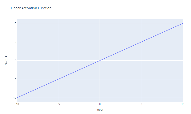
Linear activation function. Image by Author
The linear activation function is the simplest activation function, defined as:
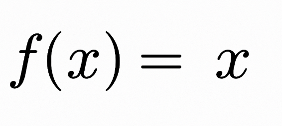
It simply returns the input x as the output. Graphically, it looks like a straight line with a slope of 1.
The main use case of the linear activation function is in the output layer of a neural network used for regression. For regression problems where we want to predict a numerical value, using a linear activation function in the output layer ensures the neural network outputs a numerical value. The linear activation function does not squash or transform the output, so the actual predicted value is returned.
However, the linear activation function is rarely used in hidden layers of neural networks. This is because it does not provide any non-linearity. The whole point of hidden layers is to learn non-linear combinations of the input features. Using a linear activation throughout would restrict the model to just learning linear transformations of the input.
Sigmoid activation
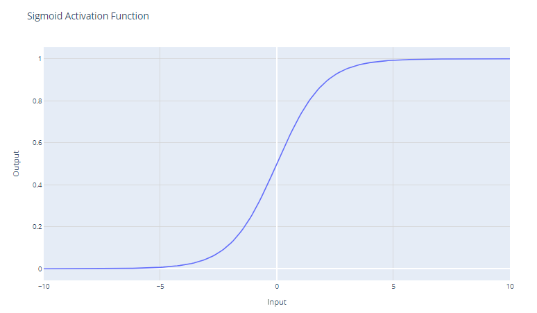
Sigmoid activation function. Image by Author
The sigmoid activation function, often represented as σ(x), is a smooth, continuously differentiable function that is historically important in the development of neural networks. The sigmoid activation function has the mathematical form:
It takes a real-valued input and squashes it to a value between 0 and 1. The sigmoid function has an "S"-shaped curve that asymptotes to 0 for large negative numbers and 1 for large positive numbers. The outputs can be easily interpreted as probabilities, which makes it natural for binary classification problems.
Sigmoid units were popular in early neural networks since the gradient is strongest when the unit's output is near 0.5, allowing efficient backpropagation training. However, sigmoid units suffer from the "vanishing gradient" problem that hampers learning in deep neural networks.
As the input values become significantly positive or negative, the function saturates at 0 or 1, with an extremely flat slope. In these regions, the gradient is very close to zero. This results in very small changes in the weights during backpropagation, particularly for neurons in the earlier layers of deep networks, which makes learning painfully slow or even halts it. This is referred to as the vanishing gradient problem in neural networks.
The main use case of the sigmoid function is as the activation for the output layer of binary classification models. It squashes the output to a probability value between 0 and 1, which can be interpreted as the probability of the input belonging to a particular class.
Tanh (hyperbolic tangent) activation
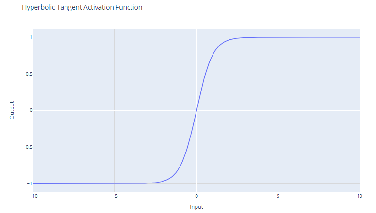
Tanh activation function. Image by Author
The tanh (hyperbolic tangent) activation function is defined as:
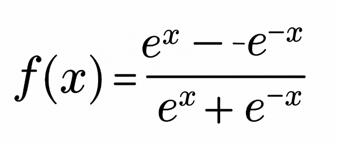
The tanh function outputs values in the range of -1 to +1. This means that it can deal with negative values more effectively than the sigmoid function, which has a range of 0 to 1.
Unlike the sigmoid function, tanh is zero-centered, which means that its output is symmetric around the origin of the coordinate system. This is often considered an advantage because it can help the learning algorithm converge faster.
Because the output of tanh ranges between -1 and +1, it has stronger gradients than the sigmoid function. Stronger gradients often result in faster learning and convergence during training because they tend to be more resilient against the problem of vanishing gradients when compared to the gradients of the sigmoid function.
Despite these advantages, the tanh function still suffers from the vanishing gradient problem. During backpropagation, the gradients of the tanh function can become very small (close to zero). This issue is particularly problematic for deep networks with many layers; the gradients of the loss function may become too small to make significant changes in the weights during training as they propagate back to the initial layers. This can drastically slow down the training process and can lead to poor convergence properties.
The tanh function is frequently used in the hidden layers of a neural network. Because of its zero-centered nature, when the data is also normalized to have mean zero, it can result in more efficient training.
If one has to choose between the sigmoid and tanh and has no specific reason to prefer one over the other, tanh is often the better choice because of the reasons mentioned above. However, the decision can also be influenced by the specific use case and the behavior of the network during initial training experiments.
You can build a Simple Neural Network from scratch using PyTorch by following our tutorial by Kurtis Pykes, or, if you are an advanced user, our Deep Learning with PyTorch course is for you. .
ReLU (rectified linear unit) activation
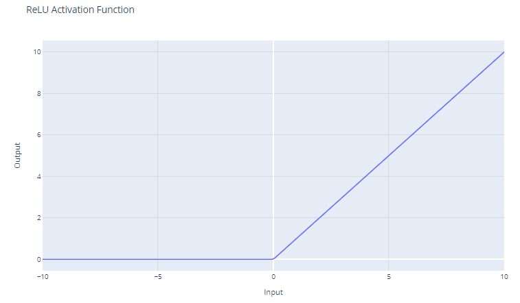
Rectified Linear Unit (ReLU) activation function. Image by Author
The Rectified Linear Unit (ReLU) activation function has the form:
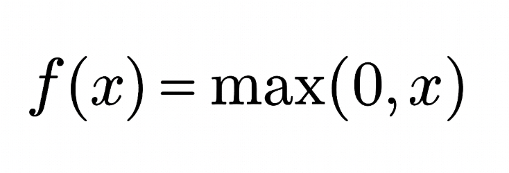
It thresholds the input at zero, returning 0 for negative values and the input itself for positive values.
For inputs greater than 0, ReLU acts as a linear function with a gradient of 1. This means that it does not alter the scale of positive inputs and allows the gradient to pass through unchanged during backpropagation. This property is critical in mitigating the vanishing gradient problem.
Even though ReLU is linear for half of its input space, it is technically a non-linear function because it has a non-differentiable point at x=0, where it abruptly changes from x. This non-linearity allows neural networks to learn complex patterns.
Since ReLU outputs zero for all negative inputs, it naturally leads to sparse activations; at any time, only a subset of neurons are activated, leading to more efficient computation.
The ReLU function is computationally inexpensive because it involves simple thresholding at zero. This allows networks to scale to many layers without a significant increase in computational burden, compared to more complex functions like tanh or sigmoid.
Softmax activation
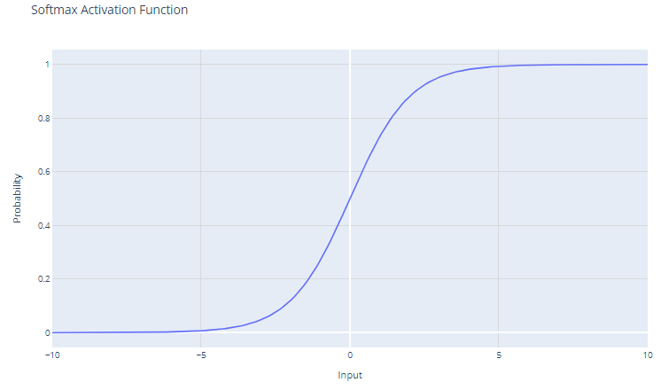
Softmax activation function. Image by Author
The softmax activation function, also known as the normalized exponential function, is particularly useful within the context of multi-class classification problems. This function operates on a vector, often referred to as the logits, which represents the raw predictions or scores for each class computed by the previous layers of a neural network.
For input vector x with elements x1, x2, ..., xC, the softmax function is defined as:
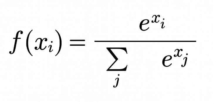
The output of the softmax function is a probability distribution that sums up to one. Each element of the output represents the probability that the input belongs to a particular class.
The use of the exponential function ensures that all output values are non-negative. This is crucial because probabilities cannot be negative.
Softmax amplifies differences in the input vector. Even small differences in the input values can lead to substantial differences in the output probabilities, with the highest input value(s) tending to dominate in the resulting probability distribution.
Softmax is typically used in the output layer of a neural network when the task involves classifying an input into one of several (more than two) possible categories (multi-class classification).
The probabilities produced by the softmax function can be interpreted as confidence scores for each class, providing insight into the model's certainty about its predictions.
Because softmax amplifies differences, it can be sensitive to outliers or extreme values. For example, if the input vector has a very large value, softmax can "squash" the probabilities of other classes, leading to an overconfident model.
Choosing the Right Activation Function
The choice of activation function depends on the type of problem you are trying to solve. Here are some guidelines:
For binary classification
Use the sigmoid activation function in the output layer. It will squash outputs between 0 and 1, representing probabilities for the two classes.
For multi-class classification
Use the softmax activation function in the output layer. It will output probability distributions over all classes.
If unsure
Use the ReLU activation function in the hidden layers. ReLU is the most common default activation function and usually a good choice.
Conclusion
We have explored the pivotal role activation functions play in the training of neural networks. We have seen how they are not just optional extras but essential elements that enable neural networks to capture and model the complexity inherent in real-world data. From the simple yet effective ReLU to the probabilistic interpretations provided by the softmax function, each activation function has its place and purpose within different layers of a network and across various problem domains.
As neural networks continue to evolve, the exploration of activation functions will undoubtedly expand, possibly including new forms that address specific challenges of emerging architectures. However, the principles and functions discussed in this blog will likely remain at the core of neural network design for the foreseeable future.
The careful selection of activation functions is a balancing act—a blend of scientific understanding and artful intuition—that can significantly affect the performance of neural networks.
Interested in learning deep learning with the Keras framework? Check out our Introduction to Deep Learning with Keras course.
FAQs
What is an activation function in a neural network?
An activation function determines whether a neuron in a neural network should be activated. It transforms the weighted sum of inputs into an output signal, introducing non-linearity that allows the network to learn complex patterns in data. Without activation functions, neural networks would only model linear relationships.
Why are activation functions important in deep learning?
Activation functions are essential in deep learning because they enable neural networks to capture non-linear relationships within data. Real-world problems—such as image recognition, speech processing, and sentiment analysis—are inherently non-linear, and activation functions like ReLU, sigmoid, and tanh make it possible to model these complexities effectively.
What are the most common types of activation functions?
The most common activation functions include ReLU (Rectified Linear Unit), Sigmoid, Tanh (Hyperbolic Tangent), Softmax, and Linear. ReLU is widely used in hidden layers for its computational efficiency, sigmoid is common for binary classification, softmax for multi-class problems, and linear activation for regression tasks.
How do I choose the right activation function for my neural network?
Choosing the right activation function depends on the task.
-
Use Sigmoid for binary classification.
-
Use Softmax for multi-class classification.
-
Use Linear for regression outputs.
-
Use ReLU (or variants like Leaky ReLU) for hidden layers. Testing different functions can help identify which one leads to faster convergence and better model performance.
What problems can occur with activation functions?
Some activation functions can lead to challenges such as the vanishing gradient problem (seen with sigmoid and tanh), where gradients become too small for effective learning. Others, like ReLU, can suffer from the dying ReLU problem, where neurons output zero and stop learning. Selecting appropriate functions and initializing weights carefully can help mitigate these issues.


