R Markdown Tutorial for Beginners

This article will explore an essential and helpful data science package that every R user needs to know—R Markdown. We'll learn what R Markdown is, what benefits it offers, what it's used for, how to install it, what capacities it provides for working with code, narrative, and data plots, what syntax it uses, the output formats for R Markdown documents, and how to render such documents and share them with our collaborators.

Since R Markdown is particularly adapted for the RStudio integrated development environment (IDE), we're going to use this IDE throughout this article. The RStudio Tutorial provides the necessary guidance on how to install RStudio and begin using it.

Let's dive in!

What is R Markdown?

R Markdown is a free and open-source R package that provides a workspace for creating data science projects. The main advantage of R Markdown is that it allows you to combine code, text, and data visualizations in a single polished, shareable, fully reproducible document that can be rendered in a wide variety of output formats, both static and interactive.

Some of its popular output formats are HTML, PDF, Microsoft Word, presentations, applications, websites, dashboards, reports, templates, articles, books, etc.

In addition, R Markdown allows easy version control tracking and supports many programming languages besides R, including Python and SQL.

If you want to dig deeper into how to author dynamic reports with R Markdown, the course Reporting with R Markdown is the right place to start.

Installing R Markdown

When using R Markdown outside of RStudio, we install it in the same way as any other R package from the Comprehensive R Archive Network (CRAN) repository:

install.packages("rmarkdown")

After installation, we need to load the package in the working R environment:

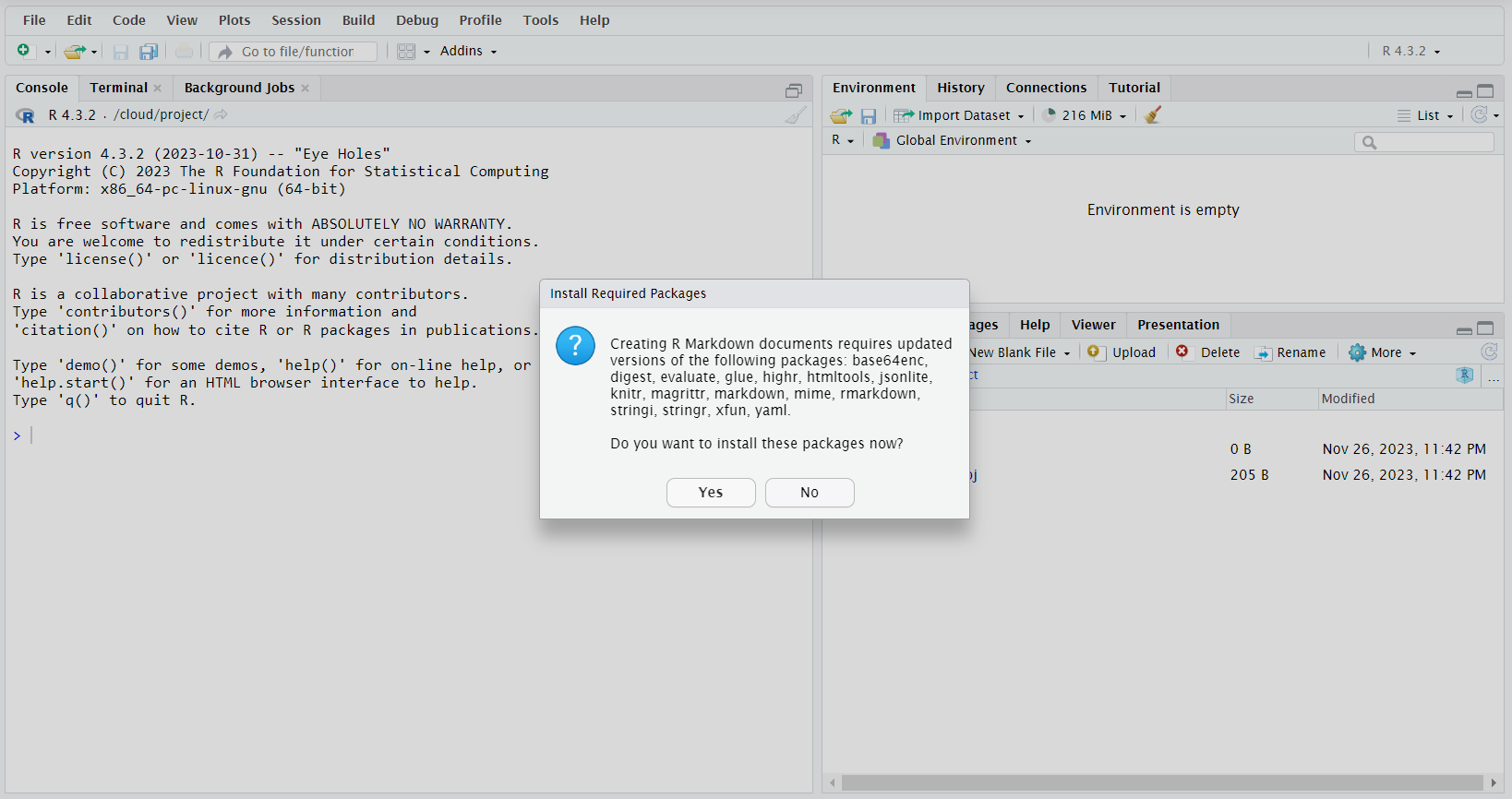
library(rmarkdown)

Instead, when working with R Markdown within RStudio—which is what we're going to do throughout this tutorial—we don't need to explicitly install and load the rmarkdown package. By clicking on File—New File—R Markdown in the menu bar of RStudio, a new R Markdown document will be opened. At this stage, we can receive a notification Install Required Packages, as follows:

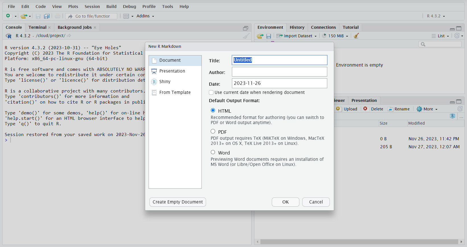
After confirming the required package installation, in a new pop-up window that appears, we provide a document title and the author's name (both optional but recommended), leave the other settings as they are, and press OK:

Default R Markdown Document

In the previous section, we opened a new R Markdown document in RStudio. It looks as follows:

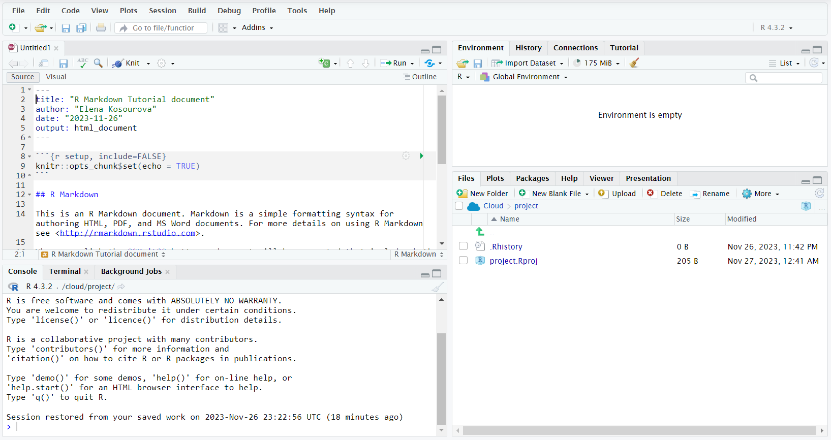
We see that it includes the title, the author's name, the current date, and the default output format that we provided in the pop-up window when opening it. Then, it’s got some examples of the basic syntax used by R Markdown, such as adding and formatting code chunks, adding headers, inserting links, emphasizing text, and generating plots.

We're going to take a more granular look at various functionalities of R Markdown and their syntax. For now, let's save this default file and then render it in the selected output format (in our case—HTML) to see what it looks like.

To save the file, we click on File—Save As... in the menu bar of RStudio.

NOTE: the name of the R Markdown document that we provided earlier is not the same as the file name. We need to save the file in the project directory and then regularly save it from time to time (File—Save) while working with it.

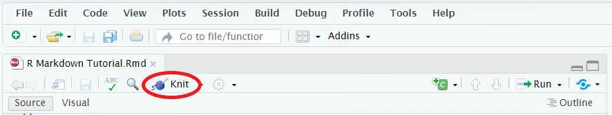
To render the saved file in the selected output format (HTML), we need to press Knit in the toolbar of the file:

Here is how our default R Markdown document looks in the HTML format:

Text Formatting in R Markdown

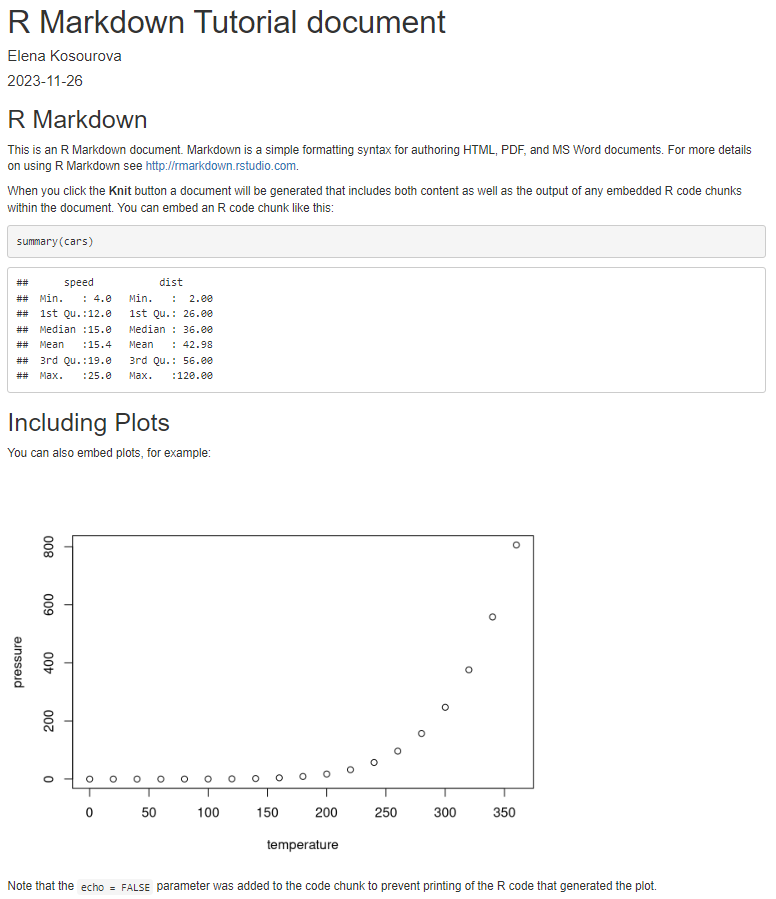
Often, text constitutes the major part of a data science project. Hence, it's important to know how to format it in R Markdown to make it easy to read, efficient, and compelling.

If you want to learn how to use R for data analysis and data science and grow both your R programming and data science skills, consider the following beginner-friendly and exhaustive career tracks:

• Data Analyst with R
• Data Scientist with R

Headers

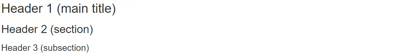
We can add various levels of headers to our R Markdown document by using the hash symbol (#). Here is the syntax:

# Header 1 (main title)

## Header 2 (section)

### Header 3 (subsection)

etc.

When rendered, the above headers will look as follows:

Text Emphasis

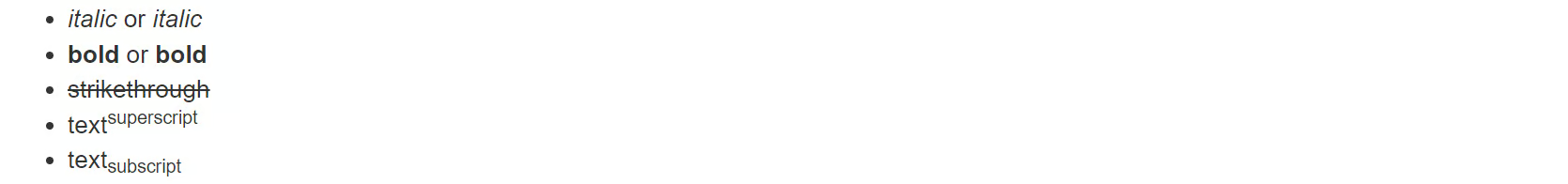
R Markdown allows to add different types of emphasis to the text, such as making it italic, bold, strikethrough, superscript, or subscript, as follows:

• *italic* or _italic_
• **bold** or __bold__
• ~~strikethrough~~
• text^superscript^
• text~subscript~

Below is how these types of emphasis appear in the rendered form:

Lists

To create an unordered list, we use one of the following three syntaxes:

* Item 1* Item 2* Item 3

or:

- Item 1- Item 2- Item 3

or:

+ Item 1+ Item 2+ Item 3

In all cases, the rendered result will be the same:

To create an ordered list, we use the following syntax:

1. Item 12. Item 23. Item 3

The rendered result will look quite the same, with an indentation added before each number.

Note that if we delete an item from an ordered list, add a new item to it, or just make an error in one of the numbers (e.g., if we write 20. instead of 2. in the above example), the numbers will be automatically corrected and shown as intended:

Block Quotes

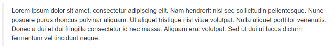
For block quotes, we use the > symbol before the first character of the text to be quoted:

> Lorem ipsum dolor sit amet, consectetur adipiscing elit. Nam hendrerit nisi sed sollicitudin pellentesque. Nunc posuere purus rhoncus pulvinar aliquam. Ut aliquet tristique nisl vitae volutpat. Nulla aliquet porttitor venenatis. Donec a dui et dui fringilla consectetur id nec massa. Aliquam erat volutpat. Sed ut dui ut lacus dictum fermentum vel tincidunt neque.

This will be rendered as:

We add an empty line after a quoted block to escape it.n unordered list of 3 items

Links

If we want to include a link as a direct path, we need to put the link path between the < and > symbols. For example, the following construction:

<https://www.google.com/>

will be rendered as:

https://www.google.com/

Instead, to anchor a link to a word or a short piece of text, we need to use the following syntax (using again the Google website as an example):

[Google](https://www.google.com/)

This will be rendered as:

Google

Images

To insert an image into our narrative, we use one of the following approaches:

1. If we want to add an image from the Internet:


2. If the image file is saved in the project folder where our R Markdown document is saved:


3. If the image file is saved on our computer but outside of the project folder:


Alt text provides short information about what it's on the picture and serves in those cases when a user is unable to see the image on the page, for whatever reason.

Let's see the first approach in action for a Pixabay picture, with the image URL https://cdn.pixabay.com/photo/2018/12/02/10/07/web-3850917_1280.jpg:


When we render the document, the picture is displayed:

Breaks

There are various types of breaks in R Markdown:

1. Line break—to start a new line. Implemented by ending the previous line with a backslash (\).
2. Paragraph break—to start a new paragraph. Implemented by ending the previous paragraph with two spaces.
3. Slide break—to start a new slide in the slide-based output formats (presentations) or a new section in all the other formats. Implemented by inserting a horizontal rule (***) into the document.
4. Page break—to start a new page, in those output formats where it's applicable, e.g., in Microsoft Word. Implemented by inserting the command \newpage into the document.

Let's put the first three types of breaks into action. Below is a piece of the Lorem ipsum text with some R Markdown break formatting symbols added to it:

Lorem ipsum dolor sit amet, consectetur adipiscing elit.\Nam hendrerit nisi sed sollicitudin pellentesque.

Nunc posuere purus rhoncus pulvinar aliquam.

***

Ut aliquet tristique nisl vitae volutpat.

Here is how it will be rendered in an HTML document:

Lorem ipsum dolor sit amet, consectetur adipiscing elit.Nam hendrerit nisi sed sollicitudin pellentesque.

Nunc posuere purus rhoncus pulvinar aliquam.

Ut aliquet tristique nisl vitae volutpat.

Code Formatting and Executing in R Markdown

Code is another essential component of any data science project. In R Markdown, we can run code (and not only in the R programming language), display both code and its output, display only code and hide its output, display only output and hide the source code, etc.

The beginner-friendly career track R Programmer and skill track R Programming are helpful resources for learning, practicing, and sharpening your R coding skills.

Code Chunks

To format and run a block of R code in R Markdown, we enclose it in a pair of triple backticks, with the first triple backticks followed by an r in braces. For example:

```{r}
print("Hello, World!")
```

If we render our document without running the code, our code chunk will look as below:

Code Language

When working with R Markdown, we aren't limited to using only R since this package also supports many other programming languages. To run a piece of code in another programming language, we provide the name of this language instead of the R in braces. Besides that, we may need to install and load some additional packages in the working R environment.

For example, to be able to use Python in R Markdown, we need to install and load the reticulate package that allows two-way communication (like creating and accessing variables) between Python and R in the same R Markdown document.

Let's rewrite the piece of code from the previous section in Python (after installing and loading the reticulate package):

```{python}
print("Hello, World!")
```

Code Chunk Execution

To execute a code chunk or the selected lines of it when working with R Markdown within RStudio, we click on the Run button on the document's toolbar and select the necessary option from the drop-down list:

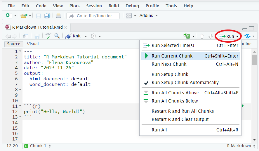
In the above picture, we see that each run option has its shortcut that we can use instead of opening every time the drop-down list.

Code Chunk Naming

While not mandatory, it's a good practice to name code chunks. It can be useful in many cases: for referencing code chunks throughout the document, code debugging, switching between code chunks, etc. Naming code chunks becomes particularly important if we work with a long document that contains a lot of code chunks.

We add the name of a code chunk in braces, right after the language name, and separate it with a white space. The name of a code chunk must not contain white spaces.

In the below example, we added the name hello_world to the chunk:

```{r hello_world}
print("Hello, World!")
```

Code Chunk Options

Code chunk options allow us to take control over code evaluation, output, decoration, cache, animation (if applicable), and plots (if applicable)—all these for each individual code chunk. We can add multiple chunk options to the same code chunk. In terms of syntax, we put chunk options in braces right after the code name (if available; otherwise, after the language name), separated from it and between themselves by a comma.

There are many chunk options available in R Markdown. Each of them has a default value, but when we decide to use them, we most probably want a value different from the default one. Let's look at the most popular chunk options and their values that could be of interest to us:

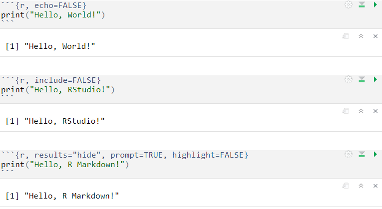
• echo=FALSE—the code itself will not be shown in the final document, only its outputs.
• eval=FALSE—the code in the code chunk will not be run.
• include=FALSE—the code chunk will be run but not included in the final document.
• results—the default value is "markup"; other values are:
• "hide"—the code output will be hidden in the final document
• "hold"—the code output will be shown with a delay, only after the whole code chunk is executed
• "asis"—the code output will be passed through without reformatting.
• message=FALSE—the messages produced by the code will not be shown.
• error=FALSE—the errors produced by the code will not be shown.
• warning=FALSE—the warnings produced by the code will not be shown.
• highlight=FALSE—the code will not be highlighted in the final document.
• prompt=TRUE—the > symbol will be added at the beginning of each code line shown in the final document.

Below are some examples of code chunks that were first run in R Markdown in RStudio and then rendered in the final document:

Code in R Markdown:

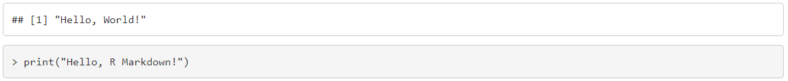
Output in the final document:

Inline Code

With inline code, we can directly insert short pieces of code into the text of our R Markdown document—they will be executed, and their outputs will be shown embedded into the text. The syntax of inline code is r <code>.

Below is a simple example of a text containing inline code:

There are `r 1+6` colors of the rainbow.

and how it is rendered in the final document:

There are 7 colors of the rainbow.

In practice, inline code is used for aggregating information about the data and helps avoid errors that can easily happen if we insert the numbers manually or if the data changes.

Plotting in R Markdown

Plotting in R Markdown implies running code that generates plots. Hence, everything that we've discussed so far about code formatting and executing in R Markdown, except for inline code, also applies to plotting. The main difference is that the output of such code will be graphics rather than just text and numbers.

The skill track Data Visualization with R will help you develop the skills needed to analyze and plot data in R and, hence, tell better data-driven stories.

To customize plots in R Markdown, like in regular R, we use the tools of R data visualization packages, as well as the plot() function of the base R.

However, to control plotting behavior in an R Markdown document, we can make use of chunk options that are related only to plotting. The majority of them are quite specific and, therefore, outside of the scope of this "getting started" tutorial. Let's thus take a look at some basic chunk options that can be helpful when plotting in R Markdown:

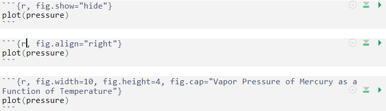
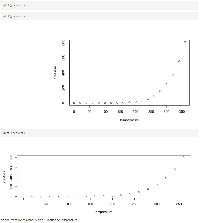
• fig.show—the default value is "asis"; other values are:
• "hide"—the plots will be generated but not included in the final document
• "hold"—the plots will be shown with a delay, only after the whole code chunk is executed
• "animate"—all the plots of the code chunk will be combined into an animation.
• fig.width—the plot width in inches, 7 by default.
• fig.height—the plot height in inches, 7 by default.
• fig.align—the way of aligning plots in the final document, can be "left", "center", or "right".
• fig.cap—a figure caption represented by a character string.
• fig.path—a path to the directory where the plot files created by the code chunk should be stored.
• fig.ext—the extension of the plot files created by the code chunk.

Below are some examples of using plotting-specific code chunks when plotting in R Markdown, including the source code and the rendered output:

Code in R Markdown:

Output in the final document:

Output Formats

Until now, we have considered only the HTML document (html_document) as an output format for the final document. However, R Markdown offers many other output formats, including Microsoft Word, Microsoft PowerPoint, PDF, interactive R notebooks, dashboards, etc.

For example, the output formats available in R Markdown for creating documents include html_document, pdf_document, word_document, github_document, html_notebook, html_vignette, etc. Instead, for creating presentations, we can use the following output formats: powerpoint_presentation, ioslides_presentation, slidy_presentation, and beamer_presentation.

To set an output format for our R Markdown document, we assign the corresponding value to the output setting in the document header (also known as the YAML header, where YAML stands for yet another markup language). For example, for our working R Markdown document, the output format is set to html_document, which is also the default output format in R Markdown:

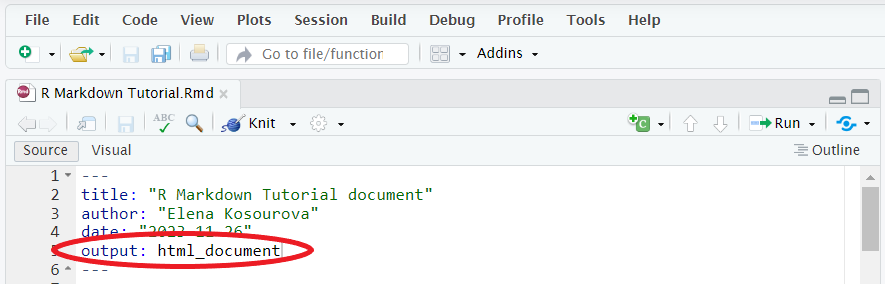
To change it, we substitute html_document with the necessary output format (pdf_document, word_document, powerpoint_presentation, etc.). Now, when we press Knit in the toolbar of the file, we'll render our document in the selected output format.

Publishing R Markdown Documents

To publish an R Markdown document, we click on File—Publish in the menu bar of RStudio and select where we want to publish it:

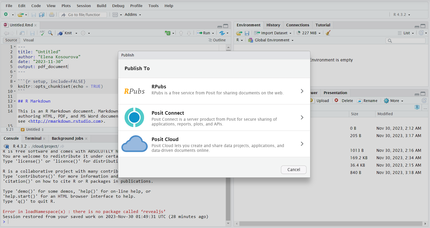
Then we follow further instructions that will depend on our previous choice and press Publish. Now, our document is ready for sharing with our collaborators.

Conclusion

To wrap up, in this article, we learned how to get started with R Markdown. First, we defined what R Markdown is and what it's used for. Then we discussed how to install R Markdown, how to format text and its various components with it, how to format and run code, how to generate plots, which output formats R Markdown offers, how to render a working document in one of those formats, and how to publish the final document for further sharing it with colleagues.

To get some hands-on practice using R Markdown, check out our Reporting with R Markdown course, which will help you reveal insights from data and author your findings as a PDF, HTML file, or Shiny app.