K-Nearest Neighbors (KNN) Classification with R Tutorial

R is a powerful tool for the implementation of KNN classification, and it is generally used by data scientists and statisticians for various machine-learning applications.

In this tutorial, we will learn about K-Nearest Neighbors, how it works, and review some advantages and disadvantages. Furthermore, we will use the 'class' and 'caret' R Package to easily implement the KNN classification model.

What is K-Nearest Neighbors?

K-Nearest Neighbors (KNN) is a supervised machine learning model that can be used for both regression and classification tasks. The algorithm is non-parametric, which means that it doesn't make any assumption about the underlying distribution of the data.

The KNN algorithm predicts the labels of the test dataset by looking at the labels of its closest neighbors in the feature space of the training dataset. The “K” is the most important hyperparameter that can be tuned to optimize the performance of the model.

KNN is a simple and intuitive algorithm that provides good results for a wide range of classification problems. It is easy to implement and understand, and it applies to both small and large datasets. However, it comes with some drawbacks too, and the main disadvantage is that it can be computationally expensive for large datasets or high-dimensional feature spaces.

The KNN algorithm is used in e-commerce recommendation engines, image recognition, fraud detection, text classification, anomaly detection, and many more. In this tutorial, we will be using the KNN algorithm for a loan approval system.

If you are confused and don’t know how to start your data science journey, take Data Scientist Professional with R career track and prepare yourself for a successful career in data science. The skill track will help you master R programming, data ingestion, data cleaning, data manipulation, data visualization, machine learning, hypothesis tests, experimental designs, SQL, and Git.

How does K-Nearest Neighbors Classification work?

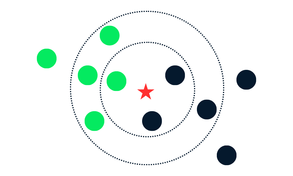
The KNN classification algorithm works by finding K neighbors (closest data points) in the training dataset to a new data point. Then, it assigns the label of the majority class among neighbors to new data points.

Let’s break down the algorithms into multiple parts.

First, it calculates the distance between the new data points and all the other data points in the training set and selects K closest points. The metric used for calculating distance can vary depending on the problems. The most used metric is the Euclidean distance.

After identifying K closest neighbors, the algorithm assigns the label of the majority class among those neighbors to the new data point. For example, if the two labels are “blue” and one label is “red” the algorithm will assign the “blue” label to a new data point.

Gif from eunsukim.me

Summary:

1. We will choose the value of K, which is the number of nearest neighbors that will be used to make the prediction.
2. Calculate the distance between that point and all the points in the training set.
3. Select the K nearest neighbors based on the distances calculated.
4. Assign the label of the majority class to the new data point.
5. Repeat steps 2 to 4 for all the data points in the test set.
6. Evaluate the accuracy of the algorithm.

The value of “K” is provided by the user, and it can be used to optimize the algorithm's performance. Smaller K values can lead to overfitting, and larger values can lead to underfitting. So, it is crucial to find optimal values that provide stability and the best fit.

Implementation of KNN in R

In this section, we will use Loan Data and train KNN classification using the class package. The dataset consists of 10,000 loans, and we will find whether a loan will be paid back based on the customer’s data.

Loading the Data

We will import the tidyverse library to access essential R packages for data loading, manipulation, and visualization. The suppressPackageStartupMessages will suppress the warnings, and you will get clean output.

After that, we will use read_csv to load the dataset, remove the “purpose” column from the dataframe using the subset function, and display the top 3 samples.

suppressPackageStartupMessages(library(tidyverse))

data <- read_csv('data/loans.csv.gz', show_col_types = FALSE)
data <- subset(data, select = -c(purpose))
head(data,3)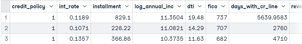

Train and Test Split

We can split the dataset manually, but using the caTools library is much cleaner.

• Set seed for reproducibility.
• Use sample.split to create an index for training and testing datasets by a 75:25 ratio.
• Use subset to create a train and test dataset, as shown below.

library(caTools)
set.seed(255)

split = sample.split(data$not_fully_paid, 
                     SplitRatio = 0.75)
train = subset(data, 
                      split == TRUE)
test = subset(data, 
                  split == FALSE)

Feature Scaling

We will now scale both the training and testing set. On the back end, the function is using (x - mean(x)) / sd(x). We are only scaling features and removing target labels from both testing and training sets.

train_scaled = scale(train[-13])
test_scaled = scale(test[-13])

Training KNN Classifier and Predicting

The class library is quite popular for training KNN classification. It is simple and fast. We will provide a scaled train and test dataset, target column, and “k” hyperparameter.

library(class)
test_pred <- knn(
                 train = train_scaled, 
                 test = test_scaled,
                 cl = train$not_fully_paid, 
                 k=10
                 )

Model Evaluation

To evaluate model results, we will display a confusion matrix using a table function. We have provided actual (test target) and predicted labels to the table function, and as we can see, we have quite good results for the majority class.

The KNN algorithm is not good at dealing with imbalanced data, and that is why we see poor performance in minority classes.

actual <- test$not_fully_paid

cm <- table(actual,test_pred)
cm

     test_pred
actual    0    1
     0 1988   23
     1  373   10

We can calculate accuracy by summing true positive values from the confusion matrix and dividing them by the total length of target columns.

As we can observe, we have good accuracy on a vanilla model. We can improve this accuracy by tuning the “K” hyperparameter and balancing the dataset.

accuracy <- sum(diag(cm))/length(actual)
sprintf("Accuracy: %.2f%%", accuracy*100)

'Accuracy: 83.46%'

KNN Classification in R using caret

In this section, we will be using caret for everything. caret is an R package for building and evaluating machine learning models. It provides an interface for major machine learning algorithms.

We will use it to split and preprocess the dataset, perform hyperparameter tuning, and train and evaluate models.

Train and Test Split

We will import the caret Package and set the seed for reproducibility. After that, we will convert the target variable from an integer to a factor. In the end, we will use createDataPartition for splitting the dataset into train and test datasets using an 80:20 ratio.

suppressPackageStartupMessages(library(caret))
set.seed(255)

data$not_fully_paid <- factor(data$not_fully_paid, levels = c(0, 1))

trainIndex <- createDataPartition(data$not_fully_paid, 
								  times=1, 
								  p = .8, 
								  list = FALSE)
train <- data[trainIndex, ]
test <- data[-trainIndex, ]

Data Preprocessing

We will then scale both the training and testing set using the preProcess function.

preProcValues <- preProcess(train, method = c("center", "scale"))
trainTransformed <- predict(preProcValues, train)
testTransformed <- predict(preProcValues, test)

Model Tuning

Before we train our KNN model, we have to find the optimal value of “K” using the training function. The train function requires a formula, scaled training dataset, model name, train control method (cross-validation), and list of hyperparameters. We are going to check model performance where “K” is 3, 5, and 7.

knnModel <- train(
		     not_fully_paid ~ ., 
		     data = trainTransformed, 
	            method = "knn", 
		     trControl = trainControl(method = "cv"), 
		     tuneGrid = data.frame(k = c(3,5,7))
		    )

Training Best Performing Model

After finding the best value of “K”, we will train the KNN classification model with a scaled training dataset.

best_model<- knn3(
                  not_fully_paid ~ .,
                  data = trainTransformed,
                  k = knnModel$bestTune$k
                 )

Model Evaluation

caret provides a simple and powerful model evaluation function. To display the model performance results, we have to first predict labels for the unseen test dataset. After that, we will use predicted and actual values to evaluate model performance using the confusionMatrix function.

predictions <- predict(best_model, testTransformed,type = "class")
# Calculate confusion matrix
cm <- confusionMatrix(predictions, testTransformed$not_fully_paid)
cm

As a result, we get the confusion matrix, model accuracy, P-Value, model sensitivity, and other important metrics that will help us determine the stability and performance of the model.

As we can see, the model has performed quite poorly on “Neg Pred Value” which is a minority class, and our balanced accuracy is 51% percent. We can get a similar result with the coin toss.

We can improve the result by balancing the classes using oversampling and undersampling methods. We can also perform feature engineering and create new features and drop highly correlated features.

Confusion Matrix and Statistics

          Reference
Prediction    0    1
         0 1570  288
         1   39   18
                                          
               Accuracy : 0.8292          
                 95% CI : (0.8116, 0.8458)
    No Information Rate : 0.8402          
    P-Value [Acc > NIR] : 0.9091          
                                          
                  Kappa : 0.0516          
                                          
 Mcnemar's Test P-Value : <2e-16          
                                          
            Sensitivity : 0.97576         
            Specificity : 0.05882         
         Pos Pred Value : 0.84499         
         Neg Pred Value : 0.31579         
             Prevalence : 0.84021         
         Detection Rate : 0.81984         
   Detection Prevalence : 0.97023         
      Balanced Accuracy : 0.51729         
                                          
       'Positive' Class : 0

We can also simplify our result by displaying it as a data frame.

data.frame(Accuracy = cm$overall["Accuracy"],
           Sensitivity = cm$byClass["Sensitivity"],
           Specificity = cm$byClass["Specificity"])

If you are a Python lover and want to learn how to perform KNN classification, read our K-Nearest Neighbors (KNN) Classification with scikit-learn tutorial to understand KNN concepts and workflow with examples.

Advantages and Disadvantages of using KNN

Advantages

1. It is a simple algorithm to understand and implement.
2. It is versatile and can be used for both regression and classification tasks.
3. It provides Interpretable results that can be visualized and understood as the predicted class is based on the labels of the nearest neighbors in the training data.
4. KNN does not make assumptions about the decision boundary between classes, and this feature allows it to capture nonlinear relationships between features.
5. The algorithm does not make assumptions about the distribution of the data, which makes it suitable for a wide range of problems.
6. KNN does not build the model. It stores the training data and uses it for prediction.

Disadvantages

1. It is computationally and memory expensive for large and complex datasets.
2. KNN performance drops for Imbalanced data. It shows biases toward the majority class, which can result in poor performance for minority classes.
3. It is not suitable for noisy data. Since the nearest neighbors of a data point may not be representative of the true class label.
4. It is not suitable for high-dimensional data, as high dimensionality can cause the distance between all data points to become similar.
5. Finding the optimal number of K neighbors can be time-consuming.
6. KNN is sensitive to outliers, as it chooses neighbors based on evidence metric.
7. It is not good at handling missing values in the training dataset.

Conclusion

In this tutorial, we have learned how to use K-Nearest Neighbors (KNN) classification with R. We have covered the basic concept of KNN and how it works. Moreover, we have learned about two libraries, class and caret, for training and evaluating KNN classification models on a real dataset.

Take the Supervised Learning in R: Classification course to learn about other supervised machine learning algorithms with R programming. You will learn about Naive Bayes, Logistic Regression, and Classification Trees with examples and code exercises.

The R tutorials involve steps for manipulation, splitting and processing the dataset, hyperparameter tuning, training the models, and evaluating the results. Due to an imbalanced dataset, we got the worst performance in the minority class.

You need to understand that the KNN algorithm is not perfect, it has some disadvantages too, and we have to take a lot of things into account before selecting it as your primary model.