K-Nearest Neighbors (KNN) Classification with scikit-learn

While kNN can be used for classification and regression, this article will focus on building a classification model. Classification in machine learning is a supervised learning task that involves predicting a categorical label for a given input data point. The algorithm is trained on a labeled dataset and uses the input features to learn the mapping between the inputs and the corresponding class labels. We can use the trained model to predict new, unseen data. You can also run the code for this tutorial by opening this DataLab workbook. 

An Overview of K-Nearest Neighbors

The kNN algorithm can be considered a voting system, where the majority class label determines the class label of a new data point among its nearest ‘k’ (where k is an integer) neighbors in the feature space. Imagine a small village with a few hundred residents, and you must decide which political party you should vote for. To do this, you might go to your nearest neighbors and ask which political party they support. If the majority of your’ k’ nearest neighbors support party A, then you would most likely also vote for party A. This is similar to how the kNN algorithm works, where the majority class label determines the class label of a new data point among its k nearest neighbors.

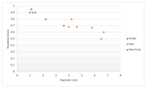
Let's take a deeper look with another example. Imagine you have data about fruit, specifically grapes and pears. You have a score for how round the fruit is and the diameter. You decide to plot these on a graph. If someone hands you a new fruit, you could plot this on the graph too, then measure the distance to k (a number) nearest points to decide what fruit it is. In the example below, if we choose to measure three points, we can say the three nearest points are pears, so I’m 100% sure this is a pear. If we choose to measure the four nearest points, three are pears while one is a grape, so we would say we are 75% sure this is a pear. We’ll cover how to find the best value for k and the different ways to measure distance later in this article.

The Dataset

To further illustrate the kNN algorithm, let's work on a case study you may find while working as a data scientist. Let's assume you are a data scientist at an online retailer, and you have been tasked with detecting fraudulent transactions. The only features you have at this stage are:

• dist_from_home: The distance between the user's home location and where the transaction was made.
• purchase_price_ratio: the ratio between the price of the item purchased in this transaction to the median purchase price of that user.

The data has 39 observations which are individual transactions. In this tutorial, we’ve been given the dataset the variable df, it looks like this:

k-Nearest Neighbors Workflow

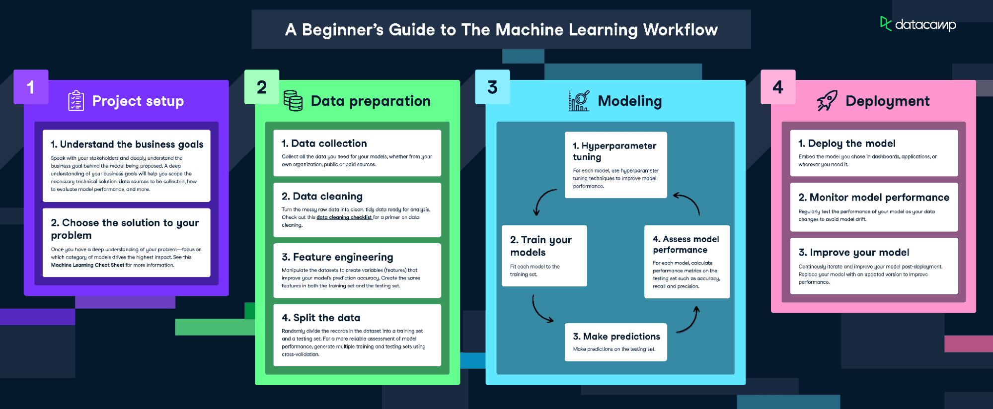
To fit and train this model, we’ll be following The Machine Learning Workflow infographic. 

Download the machine learning workflow infographic 

However, as our data is pretty clean, we won’t carry out every step. We will do the following:

• Feature engineering
• Spliting the data
• Train the model
• Hyperparameter tuning
• Assess model performance

Visualize the Data

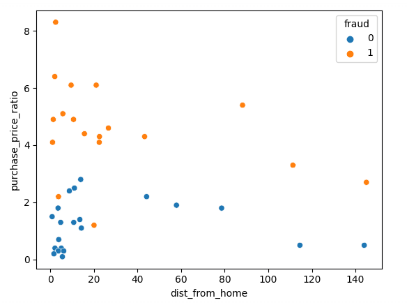
Let’s start by visualizing our data using Matplotlib; we can plot our two features in a scatterplot.

sns.scatterplot(x=df['dist_from_home'],y=df['purchase_price_ratio'], hue=df['fraud'])

As you can see, there is a clear difference between these transactions, with fraudulent transactions being of much higher value, compared to the customers' median order. The trends around distance from home are somewhat hard to interpret, with non-fraudulent transactions typically being closer to home but with several outliers. 

Normalizing & Splitting the Data

When training any machine learning model, it is important to split the data into training and test data. The training data is used to fit the model. The algorithm uses the training data to learn the relationship between the features and the target. It tries to find a pattern in the training data that can be used to make predictions on new, unseen data. The test data is used to evaluate the performance of the model. The model is tested on the test data by using it to make predictions and comparing these predictions to the actual target values. 

When training a kNN classifier, it's essential to normalize the features. This is because kNN measures the distance between points. The default is to use the Euclidean Distance, which is  the square root of the sum of the squared differences between two points. In our case, purchase_price_ratio is between 0 and 8 while dist_from_home is much larger. If we didn’t normalize this, our calculation would be heavily weighted by dist_from_home because the numbers are bigger.

We should normalize the data after splitting it into training and test sets. This is to prevent ‘data leakage’ as the normalization would give the model additional information about the test set if we normalized all the data at once.

The following code splits the data into train/test splits, then normalizes using scikit-learn’s standard scaler. We first call .fit_transform() on the training data, which fits our scaler to the mean and standard deviation of the training data. We can then apply this to the test data by calling .transform(), which uses the previously learned values.

# Split the data into features (X) and target (y)
X = df.drop('fraud', axis=1)
y = df['fraud']

# Split the data into training and test sets
X_train, X_test, y_train, y_test = train_test_split(X, y, test_size=0.2)

# Scale the features using StandardScaler
scaler = StandardScaler()
X_train = scaler.fit_transform(X_train)
X_test = scaler.transform(X_test)

Fitting and Evaluating the Model

We are now ready to train the model. For this, we’ll use a fixed value of 3 for k, but we’ll need to optimize this later on. We first create an instance of the kNN model, then fit this to our training data. We pass both the features and the target variable, so the model can learn.

knn = KNeighborsClassifier(n_neighbors=3)
knn.fit(X_train, y_train)

The model is now trained! We can make predictions on the test dataset, which we can use later to score the model.

y_pred = knn.predict(X_test)

The simplest way to evaluate this model is by using accuracy. We check the predictions against the actual values in the test set and count up how many the model got right.

accuracy = accuracy_score(y_test, y_pred)
print("Accuracy:", accuracy)

Accuracy: 0.875

This is a pretty good score! However, we may be able to do better by optimizing our value of k.

Using Cross Validation to Get the Best Value of k

Unfortunately, there is no magic way to find the best value for k. We have to loop through many different values, then use our best judgment.

In the below code, we select a range of values for k and create an empty list to store our results. We use cross-validation to find the accuracy scores, which means we don’t need to create a training and test split, but we do need to scale our data. We then loop over the values and add the scores to our list.

To implement cross-validation, we use scikit-learn’s cross_val_score. We pass an instance of the kNN model, along with our data and a number of splits to make. In the code below, we use five splits which means the model with split the data into five equal-sized groups and use 4 to train and 1 to test the result. It will loop through each group and give an accuracy score, which we average to find the best model.

k_values = [i for i in range (1,31)]
scores = []

scaler = StandardScaler()
X = scaler.fit_transform(X)

for k in k_values:
    knn = KNeighborsClassifier(n_neighbors=k)
    score = cross_val_score(knn, X, y, cv=5)
    scores.append(np.mean(score))

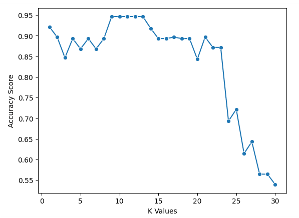
We can plot the results with the following code

sns.lineplot(x = k_values, y = scores, marker = 'o')
plt.xlabel("K Values")
plt.ylabel("Accuracy Score")

We can see from our chart that k = 9, 10, 11, 12, and 13 all have an accuracy score of just under 95%. As these are tied for the best score, it is advisable to use a smaller value for k. This is because when using higher values of k, the model will use more data points that are further away from the original. Another option would be to explore other evaluation metrics.

More Evaluation Metrics

We can now train our model using the best k value using the code below.

best_index = np.argmax(scores)
best_k = k_values[best_index]

knn = KNeighborsClassifier(n_neighbors=best_k)
knn.fit(X_train, y_train)

then evaluate with accuracy, precision, and recall (note your results may differ due to randomization)

y_pred = knn.predict(X_test)

accuracy = accuracy_score(y_test, y_pred)
precision = precision_score(y_test, y_pred)
recall = recall_score(y_test, y_pred)

print("Accuracy:", accuracy)
print("Precision:", precision)
print("Recall:", recall)

Accuracy: 0.875
Precision: 0.75
Recall: 1.0

Take it to the Next Level

• The Supervised Learning with scikit-learn course is the entry point to DataCamp's machine learning in Python curriculum and covers k-nearest neighbors.
• The Anomaly Detection in Python, Dealing with Missing Data in Python, and Machine Learning for Finance in Python courses all show examples of using k-nearest neighbors.
• The Decision Tree Classification in Python Tutorial covers another machine learning model for classifying data.
• The scikit-learn cheat sheet provides a handy reference for popular machine learning functionality.