Course
Introduction to R
4 hr
3M
Linear regression is one of the most important and foundational statistical techniques. Mastering this technique is essential for any data analyst and data scientist because, as you will see, it forms the basis for many more advanced methods.
This tutorial will guide you through the process of performing linear regression in R, which is an important programming language. By the end of this tutorial, you will understand how to implement and interpret linear regression models, making it easier to apply this knowledge to your data analysis tasks.
If you are unfamiliar with the R programming language, I recommend our tutorials to get started: Exploratory Data Analysis in R for Absolute Beginners and Mastering Data Structures in the R Programming Language.
A linear regression is a statistical model that analyzes the relationship between a response variable (often called y) and one or more variables and their interactions (often called x or explanatory variables). You make this kind of relationship in your head all the time, for example, when you calculate the age of a child based on their height, you are assuming the older they are, the taller they will be.
Linear regression is one of the most basic statistical models out there. Its results can be interpreted by almost everyone, and it has been around since the early 19th century. This is precisely what makes linear regression so popular. It’s simple, and it has survived for hundreds of years. Even though it is not as sophisticated as other algorithms like artificial neural networks or random forests, according to a survey made by KD Nuggets, regression was the algorithm most used by data scientists in 2016 and 2017. It’s even predicted that it will still be used in the year 2118!
In this linear regression tutorial, we will explore how to create a linear regression in R, looking at the steps you'll need to take with an example you can work through.
To easily run all the example code in this tutorial yourself, you can create a DataLab workbook for free that has R pre-installed and contains all code samples. For more practice on linear regression, check out our hands-on DataCamp exercise.
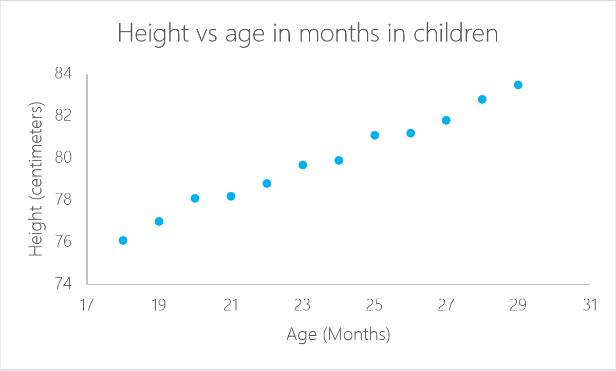
Not every problem can be solved with the same algorithm. Linear regression is known to be good when there is a linear relationship between the response and the outcome. In other words, linear regression assumes that a linear relationship exists between the response variable and the explanatory variables. In the case of two variables, this means that you can fit a line between the two variables. To look again at our previous example of the child's age, it is clear that there is a relationship between the age of children and their height.
In this particular example, you can calculate the height of a child if you know her age:

In this case, a and b are called the intercept and the slope, respectively. With the same example, a, or the intercept, is the value from where you start measuring. Newborn babies who are zero months old are not zero centimeters tall. This is the function of the intercept. The slope measures the change in height with respect to the age in months. In general, for every month older the child is, their height will increase with b.
A linear regression can be calculated in R with the command lm(). In the next example, we use this command to calculate the estimated height based on the child's age.
First, import the library readxl to read Microsoft Excel files. Our Introduction to Importing Data in R course is a great resource if you are unfamiliar with importing Excel or CSV files into an R environment like RStudio.
You can download the data to use for this tutorial before you get started. Download the data to an object called ageandheight and then create the linear regression in the third line. The lm() function takes the variables in the format:
lm([target] ~ [predictor], data = [data source])In the following code, we use the lm() function to create a linear model object, which we call lmHeight. We then use the summary() function on lmHeight in order to see detailed information on the model’s performance and coefficients.
library(readxl)
ageandheight <- read_excel("ageandheight.xls", sheet = "Hoja2") #Upload the data
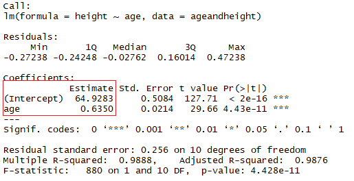
lmHeight = lm(height~age, data = ageandheight) #Create the linear regression
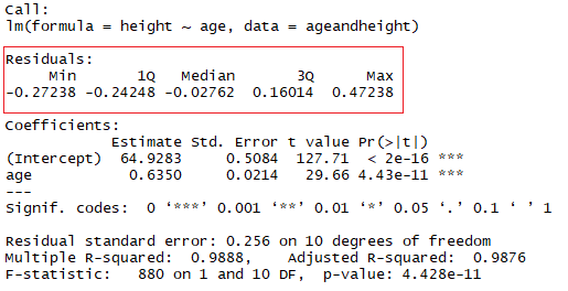
summary(lmHeight) #Review the resultsIn the red square, you can see the values of the intercept (“a” value) and the slope (“b” value) for the age. These “a” and “b” values plot a line between all the points of the data. So, in this case, if there is a child that is 20.5 months old, a is 64.92, and b is 0.635, the model predicts (on average) that its height in centimeters is around 64.92 + (0.635 * 20.5) = 77.93 cm.
When a regression takes into account two or more predictors to create the linear regression, it’s called multiple linear regression. By the same logic you used in the simple example before, the height of the child is going to be measured by:
Height = a + Age × b1 + (Number of Siblings} × b2
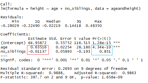
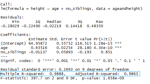
You are now looking at the height as a function of the age in months and the number of siblings the child has. In the image above, the red rectangle indicates the coefficients (b1 and b2). You can interpret these coefficients in the following way:
When comparing children with the same number of siblings, the average predicted height increases in 0.63 cm for every month the child has. The same way, when comparing children with the same age, the height decreases (because the coefficient is negative) in -0.01 cm for each increase in the number of siblings.
In R, to add another coefficient, add the symbol "+" for every additional variable you want to add to the model.
lmHeight2 = lm(height~age + no_siblings, data = ageandheight) #Create a linear regression with two variables
summary(lmHeight2) #Review the results
As you might notice already, looking at the number of siblings is a silly way to predict the height of a child. Another aspect to pay attention to in your linear models is the p-value of the coefficients. In the previous example, the blue rectangle indicates the p-values for the coefficients age and number of siblings. In simple terms, a p-value indicates whether or not you can reject or accept a hypothesis. The hypothesis, in this case, is that the predictor is not meaningful for your model.
A standard way to test if the predictors are not meaningful is by looking if the p-values are smaller than 0.05.
A good way to test the quality of the fit of the model is to look at the residuals or the differences between the real values and the predicted values. The straight line in the image above represents the predicted values. The red vertical line from the straight line to the observed data value is the residual.
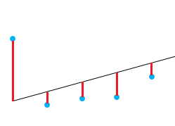
The idea here is that the sum of the residuals is approximately zero or as low as possible. In real life, most cases will not follow a perfectly straight line, so residuals are expected. In the R summary of the lm() function, you can see descriptive statistics about the residuals of the model, following the same example, the red square shows how the residuals are approximately zero.
One measure very commonly used to test how good your model is is the coefficient of determination or R². This measure is defined by the proportion of the total variability explained by the regression model.

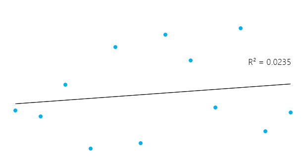
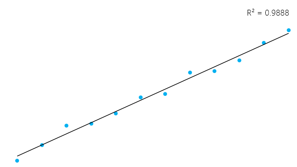
This can seem a little bit complicated, but in general, for models that fit the data well, R² is near 1. Models that poorly fit the data have R² near 0. In the examples below, the first one has an R² of 0.02; this means that the model explains only 2% of the data variability. The second one has an R² of 0.99, and the model can explain 99% of the total variability.**
However, it’s essential to keep in mind that sometimes a high R² is not necessarily good every single time (see below residual plots) and a low R² is not necessarily always bad. In real life, events don’t fit in a perfectly straight line all the time. For example, you can have in your data taller or smaller children with the same age. In some fields, an R² of 0.5 is considered good.
With the same example as above, look at the summary of the linear model to see its R².
In the blue rectangle, notice that there are two different R², one multiple and one adjusted. The multiple is the R² that you saw previously. One problem with this R² is that it cannot decrease as you add more independent variables to your model, it will continue increasing as you make the model more complex, even if these variables don’t add anything to your predictions (like the example of the number of siblings). For this reason, the adjusted R² is probably better to look at if you are adding more than one variable to the model since it only increases if it reduces the overall error of the predictions.
You can have a pretty good R² in your model, but let’s not rush to conclusions here. Let’s see an example. You are going to predict the pressure of a material in a laboratory based on its temperature.
Let’s plot the data (in a simple scatterplot) and add the line you built with your linear model. In this example, let R read the data first, again with the read_excel command, to create a dataframe with the data, then create a linear regression with your new data. The command plot() takes a data frame and plots the variables on it. In this case, it plots the pressure against the temperature of the material. Then, add the line made by the linear regression with the command abline.
pressure <- read_excel("pressure.xlsx") #Upload the data
lmTemp = lm(Pressure~Temperature, data = pressure) #Create the linear regression
plot(pressure, pch = 16, col = "blue") #Plot the results
abline(lmTemp) #Add a regression line
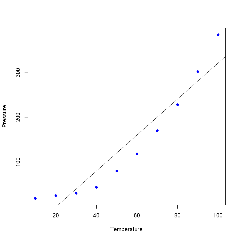
If you see the summary of your new model, you can see that it has pretty good results (look at the R²and the adjusted R²)
summary(lmTemp)
Call:
lm(formula = Pressure ~ Temperature, data = pressure)

Residuals:
   Min     1Q Median     3Q    Max
-41.85 -34.72 -10.90  24.69  63.51

Coefficients:
            Estimate Std. Error t value Pr(>|t|)
(Intercept) -81.5000    29.1395  -2.797   0.0233 *
Temperature   4.0309     0.4696   8.583 2.62e-05 ***
---
Signif. codes:  0 '***' 0.001 '**' 0.01 '*' 0.05 '.' 0.1 ' ' 1

Residual standard error: 42.66 on 8 degrees of freedom
Multiple R-squared:  0.902,    Adjusted R-squared:  0.8898
F-statistic: 73.67 on 1 and 8 DF,  p-value: 2.622e-05
Ideally, when you plot the residuals, they should look random. Otherwise means that maybe there is a hidden pattern that the linear model is not considering. To plot the residuals, use the command plot(lmTemp$residuals).
plot(lmTemp$residuals, pch = 16, col = "red")
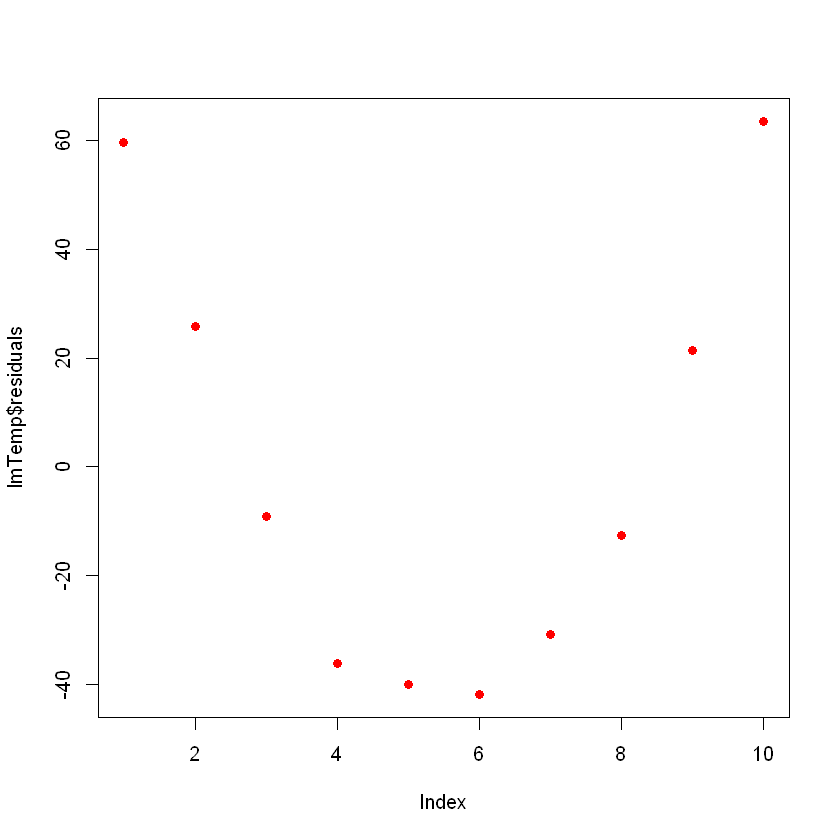
This can be a problem. If you have more data, your simple linear model will not be able to generalize well. In the previous picture, notice that there is a pattern (like a curve on the residuals). This is not random at all.
What you can do is a transformation of the variable. Many possible transformations can be performed on your data, such as adding a quadratic term (x2), a cubic (x3), or even more complex such as ln(X), ln(X+1), sqrt(X), 1/x, Exp(X). The choice of the correct transformation will come with some knowledge of algebraic functions, practice, trial, and error.
Let’s try with a quadratic term. For this, add the term “I” (capital "I") before your transformation, for example, this will be the normal linear regression formula:
lmTemp2 = lm(Pressure~Temperature + I(Temperature^2), data = pressure) #Create a linear regression with a quadratic coefficient
summary(lmTemp2) #Review the results
Call:
lm(formula = Pressure ~ Temperature + I(Temperature^2), data = pressure)

Residuals:
    Min      1Q  Median      3Q     Max
-4.6045 -1.6330  0.5545  1.1795  4.8273

Coefficients:
                  Estimate Std. Error t value Pr(>|t|)
(Intercept)      33.750000   3.615591   9.335 3.36e-05 ***
Temperature      -1.731591   0.151002 -11.467 8.62e-06 ***
I(Temperature^2)  0.052386   0.001338  39.158 1.84e-09 ***
---
Signif. codes:  0 '***' 0.001 '**' 0.01 '*' 0.05 '.' 0.1 ' ' 1

Residual standard error: 3.074 on 7 degrees of freedom
Multiple R-squared:  0.9996,    Adjusted R-squared:  0.9994
F-statistic:  7859 on 2 and 7 DF,  p-value: 1.861e-12
Notice that the model improved significantly. If you plot the residuals of the new model, they will look like this:
plot(lmTemp2$residuals, pch = 16, col = "red")
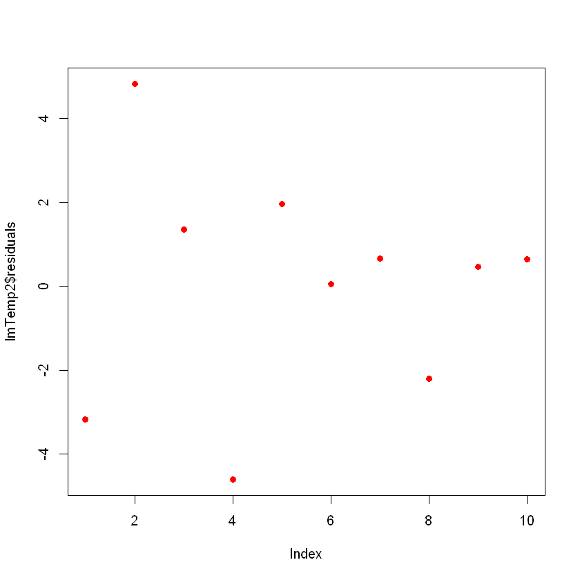
Now you don’t see any clear patterns on your residuals, which is good!
In your data, you may have influential points that might skew your model, sometimes unnecessarily. Think of a mistake in the data entry, and instead of writing “2.3” the value was “23”. The most common kind of influential point are the outliers, which are data points where the observed response does not appear to follow the pattern established by the rest of the data.
You can detect influential points by looking at the object containing the linear model, using the function cooks.distance() and then plot these distances. Change a value on purpose to see how it looks on the Cooks Distance plot. To change a specific value, you can directly point at it with ageandheight[row number, column number] = [new value]. In this case, the height is changed to 7.7 of the second example:
ageandheight[2, 2] = 7.7
head(ageandheight)
| age | height | no_siblings |
|---|---|---|
| 18 | 76.1 | 0 |
| 19 | 7.7 | 2 |
| 20 | 78.1 | 0 |
| 21 | 78.2 | 3 |
| 22 | 78.8 | 4 |
| 23 | 79.7 | 1 |
You create the model again and see how the summary is giving a bad fit, and then plot the Cooks Distances. For this, after creating the linear regression, use the command cooks.distance([linear model] , and then, if you want, you can plot these distances with the command plot().
lmHeight3 = lm(height~age, data = ageandheight)#Create the linear regression
summary(lmHeight3)#Review the results
plot(cooks.distance(lmHeight3), pch = 16, col = "blue") #Plot the Cooks Distances.
Call:
lm(formula = height ~ age, data = ageandheight)

Residuals:
    Min      1Q  Median      3Q     Max
-53.704  -2.584   3.609   9.503  17.512

Coefficients:
            Estimate Std. Error t value Pr(>|t|)
(Intercept)    7.905     38.319   0.206    0.841
age            2.816      1.613   1.745    0.112

Residual standard error: 19.29 on 10 degrees of freedom
Multiple R-squared:  0.2335,    Adjusted R-squared:  0.1568
F-statistic: 3.046 on 1 and 10 DF,  p-value: 0.1115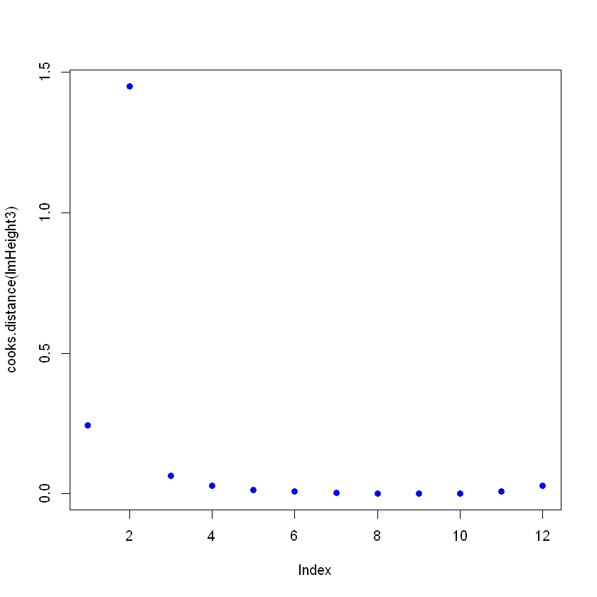
Notice that there is a point that does not follow the pattern, and it might be affecting the model. Here you can make decisions on this point, in general, there are three reasons why a point is so influential:
If the case is 1 or 2, then you can remove the point (or correct it). If it's 3, it's not worth deleting a valid point; maybe you can try on a non-linear model rather than a linear model like linear regression.
Beware that an influential point can be a valid point, be sure to check the data and its source before deleting it. It’s common to see in statistics books this quote: “Sometimes we throw out perfectly good data when we should be throwing out questionable models.”
You made it to the end! Linear regression is a big topic, and it's here to stay. Here, we've presented a few tricks that can help to tune and take the most advantage of such a powerful yet simple algorithm. You also learned how to understand what's behind this simple statistical model and how you can modify it according to your needs. You can also explore other options by typing ?lm on the R console and looking at the different parameters not covered here. Check out our Regularization Tutorial: Ridge, Lasso and Elastic Net. If you are interested in diving into statistical models, go ahead and check the course on Statistical Modeling in R.
As linear regression forms the foundation of many advanced analytical techniques, ensuring your team has a strong grasp of this and other essential skills is crucial for long-term success.
DataCamp for Business provides a tailored solution for organizations looking to upskill their teams in data science and analytics. With custom learning paths and practical, hands-on courses that cover a wide range of statistical methods, including regression and predictive modeling, your team can confidently handle complex data challenges.
Request a demo today and invest in the future of your organization by enabling your team to stay current with the latest tools and techniques in data analysis.
Our certification programs help you stand out and prove your skills are job-ready to potential employers.

R Courses
Course
Course
Course
Tutorial
Zoumana Keita
Tutorial
Josef Waples
Tutorial
Vidhi Chugh
Tutorial
DataCamp Team
Tutorial
Karlijn Willems
Tutorial
Samuel Shaibu
