Course
Introduction to R
4 hr
3M
Run and edit the code from this tutorial online
Run codeWe are going to cover both mathematical properties of the methods as well as practical R examples, plus some extra tweaks and tricks. Without further ado, let's get started!
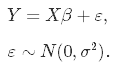
Let's kick off with the basics: the simple linear regression model, in which you aim at predicting n observations of the response variable, Y, with a linear combination of m predictor variables, X, and a normally distributed error term with variance σ2:
As we don't know the true parameters, β, we have to estimate them from the sample. In the Ordinary Least Squares (OLS) approach, we estimate them as $\hat\beta$ in such a way, that the sum of squares of residuals is as small as possible. In other words, we minimize the following loss function:
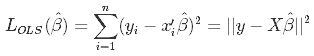
in order to obtain the infamous OLS parameter estimates, $\hat\beta_{OLS} = (X'X)^{-1}(X'Y)$.
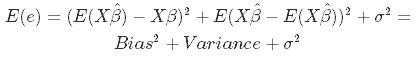
In statistics, there are two critical characteristics of estimators to be considered: the bias and the variance. The bias is the difference between the true population parameter and the expected estimator:
It measures the accuracy of the estimates. Variance, on the other hand, measures the spread, or uncertainty, in these estimates. It is given by
where the unknown error variance σ2 can be estimated from the residuals as
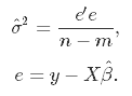
This graphic illustrates what bias and variance are. Imagine the bull's-eye is the true population parameter that we are estimating, β, and the shots at it are the values of our estimates resulting from four different estimators - low bias and variance, high bias and variance, and the combinations thereof.
Source: kdnuggets.com
Both the bias and the variance are desired to be low, as large values result in poor predictions from the model. In fact, the model's error can be decomposed into three parts: error resulting from a large variance, error resulting from significant bias, and the remainder - the unexplainable part.
The OLS estimator has the desired property of being unbiased. However, it can have a huge variance. Specifically, this happens when:
The general solution to this is: reduce variance at the cost of introducing some bias. This approach is called regularization and is almost always beneficial for the predictive performance of the model. To make it sink in, let's take a look at the following plot.
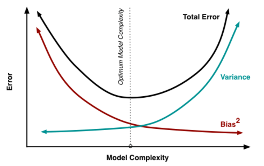
Source: researchgate.net
As the model complexity, which in the case of linear regression can be thought of as the number of predictors, increases, estimates' variance also increases, but the bias decreases. The unbiased OLS would place us on the right-hand side of the picture, which is far from optimal. That's why we regularize: to lower the variance at the cost of some bias, thus moving left on the plot, towards the optimum.
From the discussion so far we have concluded that we would like to decrease the model complexity, that is the number of predictors. We could use the forward or backward selection for this, but that way we would not be able to tell anything about the removed variables' effect on the response. Removing predictors from the model can be seen as settings their coefficients to zero. Instead of forcing them to be exactly zero, let's penalize them if they are too far from zero, thus enforcing them to be small in a continuous way. This way, we decrease model complexity while keeping all variables in the model. This, basically, is what Ridge Regression does.
In Ridge Regression, the OLS loss function is augmented in such a way that we not only minimize the sum of squared residuals but also penalize the size of parameter estimates, in order to shrink them towards zero:
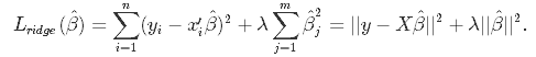
Solving this for $\hat\beta$ gives the the ridge regression estimates $\hat\beta_{ridge} = (X'X+\lambda I)^{-1}(X'Y)$, where I denotes the identity matrix.
The λ parameter is the regularization penalty. We will talk about how to choose it in the next sections of this tutorial, but for now notice that:
So, setting λ to 0 is the same as using the OLS, while the larger its value, the stronger is the coefficients' size penalized.
Incorporating the regularization coefficient in the formulas for bias and variance gives us
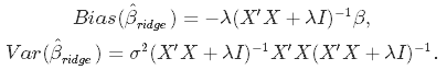
From there you can see that as λ becomes larger, the variance decreases, and the bias increases. This poses the question: how much bias are we willing to accept in order to decrease the variance? Or: what is the optimal value for λ?
There are two ways we could tackle this issue. A more traditional approach would be to choose λ such that some information criterion, e.g., AIC or BIC, is the smallest. A more machine learning-like approach is to perform cross-validation and select the value of λ that minimizes the cross-validated sum of squared residuals (or some other measure). The former approach emphasizes the model's fit to the data, while the latter is more focused on its predictive performance. Let's discuss both.
Minimizing Information Criteria
This approach boils down to estimating the model with many different values for λ and choosing the one that minimizes the Akaike or Bayesian Information Criterion:

where dfridge is the number of degrees of freedom. Watch out here! The number of degrees of freedom in ridge regression is different than in the regular OLS! This is often overlooked which leads to incorrect inference. In both OLS and ridge regression, degrees of freedom are equal to the trace of the so-called hat matrix, which is a matrix that maps the vector of response values to the vector of fitted values as follows: $\hat y = H y$.
In OLS, we find that HOLS = X(X′X)−1X, which gives dfOLS = trHOLS = m, where m is the number of predictor variables. In ridge regression, however, the formula for the hat matrix should include the regularization penalty: Hridge = X(X′X + λI)−1X, which gives dfridge = trHridge, which is no longer equal to m. Some ridge regression software produce information criteria based on the OLS formula. To be sure you are doing things right, it is safer to compute them manually, which is what we will do later in this tutorial.
Minimizing cross-validated residuals
To choose λ through cross-validation, you should choose a set of P values of λ to test, split the dataset into K folds, and follow this algorithm:
Of course, no need to program it yourself - R has all the dedicated functions.
In R, the glmnet package contains all you need to implement ridge regression. We will use the infamous mtcars dataset as an illustration, where the task is to predict miles per gallon based on car's other characteristics. One more thing: ridge regression assumes the predictors are standardized and the response is centered! You will see why this assumption is needed in a moment. For now, we will just standardize before modeling.
# Load libraries, get data & set seed for reproducibility ---------------------
set.seed(123)    # seef for reproducibility
library(glmnet)  # for ridge regression
library(dplyr)   # for data cleaning
library(psych)   # for function tr() to compute trace of a matrix

data("mtcars")
# Center y, X will be standardized in the modelling function
y <- mtcars %>% select(mpg) %>% scale(center = TRUE, scale = FALSE) %>% as.matrix()
X <- mtcars %>% select(-mpg) %>% as.matrix()


# Perform 10-fold cross-validation to select lambda ---------------------------
lambdas_to_try <- 10^seq(-3, 5, length.out = 100)
# Setting alpha = 0 implements ridge regression
ridge_cv <- cv.glmnet(X, y, alpha = 0, lambda = lambdas_to_try,
                      standardize = TRUE, nfolds = 10)
# Plot cross-validation results
plot(ridge_cv)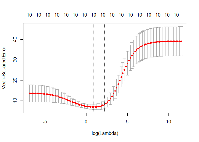
# Best cross-validated lambda
lambda_cv <- ridge_cv$lambda.min
# Fit final model, get its sum of squared residuals and multiple R-squared
model_cv <- glmnet(X, y, alpha = 0, lambda = lambda_cv, standardize = TRUE)
y_hat_cv <- predict(model_cv, X)
ssr_cv <- t(y - y_hat_cv) %*% (y - y_hat_cv)
rsq_ridge_cv <- cor(y, y_hat_cv)^2


# Use information criteria to select lambda -----------------------------------
X_scaled <- scale(X)
aic <- c()
bic <- c()
for (lambda in seq(lambdas_to_try)) {
  # Run model
  model <- glmnet(X, y, alpha = 0, lambda = lambdas_to_try[lambda], standardize = TRUE)
  # Extract coefficients and residuals (remove first row for the intercept)
  betas <- as.vector((as.matrix(coef(model))[-1, ]))
  resid <- y - (X_scaled %*% betas)
  # Compute hat-matrix and degrees of freedom
  ld <- lambdas_to_try[lambda] * diag(ncol(X_scaled))
  H <- X_scaled %*% solve(t(X_scaled) %*% X_scaled + ld) %*% t(X_scaled)
  df <- tr(H)
  # Compute information criteria
  aic[lambda] <- nrow(X_scaled) * log(t(resid) %*% resid) + 2 * df
  bic[lambda] <- nrow(X_scaled) * log(t(resid) %*% resid) + 2 * df * log(nrow(X_scaled))
}

# Plot information criteria against tried values of lambdas
plot(log(lambdas_to_try), aic, col = "orange", type = "l",
     ylim = c(190, 260), ylab = "Information Criterion")
lines(log(lambdas_to_try), bic, col = "skyblue3")
legend("bottomright", lwd = 1, col = c("orange", "skyblue3"), legend = c("AIC", "BIC"))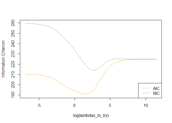
# Optimal lambdas according to both criteria
lambda_aic <- lambdas_to_try[which.min(aic)]
lambda_bic <- lambdas_to_try[which.min(bic)]

# Fit final models, get their sum of squared residuals and multiple R-squared
model_aic <- glmnet(X, y, alpha = 0, lambda = lambda_aic, standardize = TRUE)
y_hat_aic <- predict(model_aic, X)
ssr_aic <- t(y - y_hat_aic) %*% (y - y_hat_aic)
rsq_ridge_aic <- cor(y, y_hat_aic)^2

model_bic <- glmnet(X, y, alpha = 0, lambda = lambda_bic, standardize = TRUE)
y_hat_bic <- predict(model_bic, X)
ssr_bic <- t(y - y_hat_bic) %*% (y - y_hat_bic)
rsq_ridge_bic <- cor(y, y_hat_bic)^2


# See how increasing lambda shrinks the coefficients --------------------------
# Each line shows coefficients for one variables, for different lambdas.
# The higher the lambda, the more the coefficients are shrinked towards zero.
res <- glmnet(X, y, alpha = 0, lambda = lambdas_to_try, standardize = FALSE)
plot(res, xvar = "lambda")
legend("bottomright", lwd = 1, col = 1:6, legend = colnames(X), cex = .7)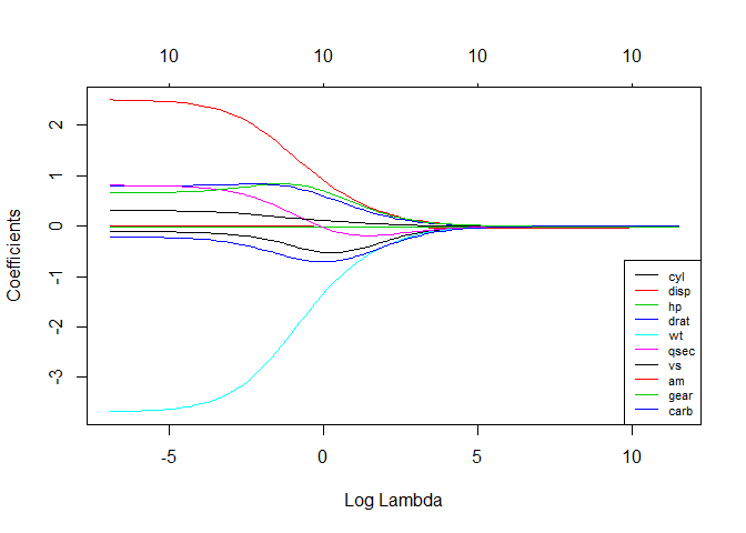
I have mentioned before that ridge regression assumes the predictors to be scaled to z-scores. Why is this required? This scaling ensures that the penalty term penalizes each coefficient equally so that it takes the form $\lambda \sum_{j=1}^m\hat\beta_j^2$. If the predictors are not standardized, their standard deviations are not all equal to one, and it can be shown with some math that this results in a penalty term of the form $\lambda \sum_{j=1}^m\hat\beta_j^2/std(x_j)$. So, the unstandardized coefficients are then weighted by the inverse of the standard deviations of their corresponding predictors. We scale the X matrix to avoid this, but... Instead of solving this heteroskedasticity problem by equalizing the variances of all predictors via scaling, we could just as well use them as weights in the estimation process! This is the idea behind the Differentially-weighted or Heteroskedastic Ridge Regression.
The idea is to penalize different coefficients with different strength by introducing weights to the loss function:
How to choose the weights wj? Run a set of univariate regressions (response vs. one of the predictors) for all predictors, extract the estimate of the coefficient's variance, $\hat\sigma_{j}$, and use it as the weight! This way:
Here is how to do this in R. As this method is not implemented in glmnet, we would need a bit of programming here.
# Calculate the weights from univariate regressions
weights <- sapply(seq(ncol(X)), function(predictor) {
uni_model <- lm(y ~ X[, predictor])
coeff_variance <- summary(uni_model)$coefficients[2, 2]^2
})
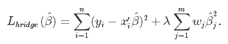
# Heteroskedastic Ridge Regression loss function - to be minimized
hridge_loss <- function(betas) {
sum((y - X %*% betas)^2) + lambda * sum(weights * betas^2)
}
# Heteroskedastic Ridge Regression function
hridge <- function(y, X, lambda, weights) {
# Use regular ridge regression coefficient as initial values for optimization
model_init <- glmnet(X, y, alpha = 0, lambda = lambda, standardize = FALSE)
betas_init <- as.vector(model_init$beta)
# Solve optimization problem to get coefficients
coef <- optim(betas_init, hridge_loss)$par
# Compute fitted values and multiple R-squared
fitted <- X %*% coef
rsq <- cor(y, fitted)^2
names(coef) <- colnames(X)
output <- list("coef" = coef,
"fitted" = fitted,
"rsq" = rsq)
return(output)
}
# Fit model to the data for lambda = 0.001
hridge_model <- hridge(y, X, lambda = 0.001, weights = weights)
rsq_hridge_0001 <- hridge_model$rsq
# Cross-validation or AIC/BIC can be employed to select some better lambda!
# You can find some useful functions for this at https://github.com/MichalOleszak/momisc/blob/master/R/hridge.RLasso, or Least Absolute Shrinkage and Selection Operator, is quite similar conceptually to ridge regression. It also adds a penalty for non-zero coefficients, but unlike ridge regression which penalizes sum of squared coefficients (the so-called L2 penalty), lasso penalizes the sum of their absolute values (L1 penalty). As a result, for high values of λ, many coefficients are exactly zeroed under lasso, which is never the case in ridge regression.
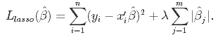
The only difference in ridge and lasso loss functions is in the penalty terms. Under lasso, the loss is defined as:
To run Lasso Regression you can re-use the glmnet() function, but with the alpha parameter set to 1.
# Perform 10-fold cross-validation to select lambda ---------------------------
lambdas_to_try <- 10^seq(-3, 5, length.out = 100)
# Setting alpha = 1 implements lasso regression
lasso_cv <- cv.glmnet(X, y, alpha = 1, lambda = lambdas_to_try,
                      standardize = TRUE, nfolds = 10)
# Plot cross-validation results
plot(lasso_cv)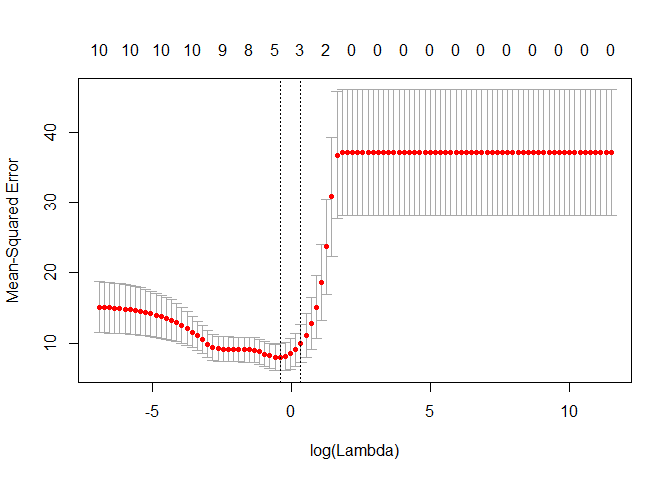
# Best cross-validated lambda
lambda_cv <- lasso_cv$lambda.min
# Fit final model, get its sum of squared residuals and multiple R-squared
model_cv <- glmnet(X, y, alpha = 1, lambda = lambda_cv, standardize = TRUE)
y_hat_cv <- predict(model_cv, X)
ssr_cv <- t(y - y_hat_cv) %*% (y - y_hat_cv)
rsq_lasso_cv <- cor(y, y_hat_cv)^2


# See how increasing lambda shrinks the coefficients --------------------------
# Each line shows coefficients for one variables, for different lambdas.
# The higher the lambda, the more the coefficients are shrinked towards zero.
res <- glmnet(X, y, alpha = 1, lambda = lambdas_to_try, standardize = FALSE)
plot(res, xvar = "lambda")
legend("bottomright", lwd = 1, col = 1:6, legend = colnames(X), cex = .7)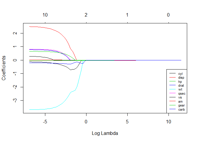
Let us compare the multiple R-squared of various models we have estimated!
rsq <- cbind("R-squared" = c(rsq_ridge_cv, rsq_ridge_aic, rsq_ridge_bic, rsq_hridge_0001, rsq_lasso_cv))
rownames(rsq) <- c("ridge cross-validated", "ridge AIC", "ridge BIC", "hridge 0.001", "lasso cross_validated")
print(rsq)

##                       R-squared
## ridge cross-validated 0.8536968
## ridge AIC             0.8496310
## ridge BIC             0.8412011
## hridge 0.001          0.7278277
## lasso cross_validated 0.8426777
They seem to perform similarly for these data. Remember, that the heteroskedastic model is untuned, and the lambda is not optimal! Some more general considerations about how ridge and lasso compare:
Elastic Net first emerged as a result of critique on lasso, whose variable selection can be too dependent on data and thus unstable. The solution is to combine the penalties of ridge regression and lasso to get the best of both worlds. Elastic Net aims at minimizing the following loss function:
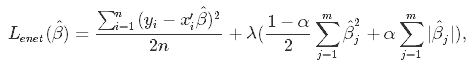
where α is the mixing parameter between ridge (α = 0) and lasso (α = 1).
Now, there are two parameters to tune: λ and α. The glmnet package allows to tune λ via cross-validation for a fixed α, but it does not support α-tuning, so we will turn to caret for this job.
library(caret)

# Set training control
train_control <- trainControl(method = "repeatedcv",
                              number = 5,
                              repeats = 5,
                              search = "random",
                              verboseIter = TRUE)

# Train the model
elastic_net_model <- train(mpg ~ .,
                           data = cbind(y, X),
                           method = "glmnet",
                           preProcess = c("center", "scale"),
                           tuneLength = 25,
                           trControl = train_control)

# Check multiple R-squared
y_hat_enet <- predict(elastic_net_model, X)
rsq_enet <- cor(y, y_hat_enet)^2Congratulations! If you have made it up to this point, you already know that:
If you want to learn more about regression in R, take DataCamp's Supervised Learning in R: Regression course. Also check out our Linear Regression in R and Logistic Regression in R tutorials.
R Courses
Course
Course
Course
Tutorial
Eladio Montero Porras
Tutorial
DataCamp Team
Tutorial
Zoumana Keita
Tutorial
Vidhi Chugh
Tutorial
Francisco Lima
Tutorial
Sayak Paul