Course

Introduction to Neural Networks
Neural networks or simulated neural networks are a subset of machine learning which is inspired by the human brain. They mimic how biological neurons communicate with one another to come up with a decision.
A neural network consists of an input layer, a hidden layer, and an output layer. The first layer receives raw input, it is processed by multiple hidden layers, and the last layer produces the result.
In the example below, we have simulated the training process of neural networks to classify tabular data. We have parameters X1 and X2 that are passed through 2 hidden layers of 4 and 2 neurons to produce output. With multiple iterations, the model is getting better at classifying the targets.
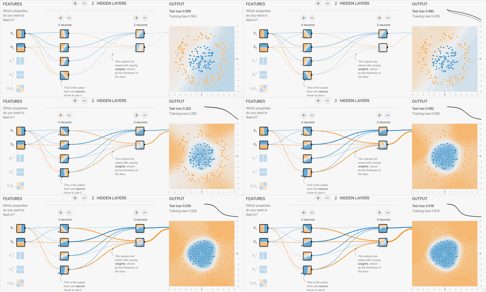
Image created with TF Playground
Deep learning algorithms or deep neural networks consist of multiple hidden layers and nodes. The “deep” means the depth of neural networks. They are generally used for solving complex problems such as Image classification, Speech recognition, and Text generation.
Learn more about neural networks by reading our Deep Learning Tutorial. You will learn how Activation Function, Loss Function, and Backpropagation work to produce accurate results.
Types of Neural Networks
Multiple types of neural networks are used for advanced machine-learning applications. We don’t have one model architecture that works for all. The oldest type of neural network is known as Perceptron, created by Frank Rosenblatt in 1958.
In this section, we will cover the 5 most popular types of neural networks used in the tech industry.
Feedforward Neural Networks
Feedforward neural networks consist of an input layer, hidden layers, and an output layer. It is called feedforward because the data flow in the forward direction, and there is no backpropagation. It is mostly used in Classification, Speech recognition, Face recognition, and Pattern recognition.
Multi-Layer Perceptron
Multi-Layer Perceptrons (MLPs) solve shortcomings of the feedforward neural network of not being able to learn through backpropagation. It is bidirectional and consists of multiple hidden layers and activation functions. MLPs use forward propagation for inputs and backpropagation for updating the weights. They are basic neural networks that have laid the foundation for computer vision, language technology, and other neural networks.
Note: MLPs consist of sigmoid neurons, not perceptrons, because real-world problems are non-liners.
Convolutional Neural Networks (CNNs)
Convolution Neural Networks (CNN) are generally used in computer vision, image recognition, and pattern recognition. It is used for extracting important features from the image using multiple convolutional layers. The convolutional layer in CNN uses a custom matrix (filter) to convolute over images and create a map.
Generally, Convolution Neural Networks consist of the input layer, convolution layer, pooling layer, fully connected layer, and output layer. Read our Python Convolutional Neural Networks (CNN) with TensorFlow tutorial to learn more about how CNN works.
Recurrent Neural Networks (RNNs)
Recurrent Neural Networks (RNNs) are commonly used for sequential data such as texts, sequences of images, and time series. They are similar to feed-forward networks, except they get inputs from previous sequences using a feedback loop. RNNs are used in NLP, sales predictions, and weather forecasting.
RNNs come with vanishing gradient problems, which are solved by advanced versions of RNNs called Short-Term Memory Networks (LSTMs) and Gated Recurrent Unit Networks (GRUs). Read Recurrent Neural Network Tutorial (RNN) tutorial to learn more about LSTMs and GRUs.
Implementation of Neural Networks in R
We will learn to create neural networks with popular R packages neuralnet and Keras.
In the first example, we will create a simple neural network with minimum effort, and in the second example, we will tackle a more advanced problem using the Keras package.
Let's set up the R environment by downloading essential libraries and dependencies.
install.packages(c('neuralnet','keras','tensorflow'),dependencies = T)Simple Neural Network implementation in R
In this first example, we will be using built-in R data iris and solve multi-classification problems with a simple neural network.
We will start by importing essential R packages for data manipulation and model training.
library(tidyverse)
library(neuralnet)
Data Analysis
You can access data by typing `iris` and running it in the R console. Before training the data, we need to convert character column types into factors.
Note: we are using the DataCamp R workspace for running the examples.
iris <- iris %>% mutate_if(is.character, as.factor)The `summary` function is used for statistical analysis and data distribution.
summary(iris)As we can see, we have balanced data. All three target classes have 50 samples.
Sepal.Length    Sepal.Width     Petal.Length    Petal.Width
Min.   :4.300   Min.   :2.000   Min.   :1.000   Min.   :0.100
1st Qu.:5.100   1st Qu.:2.800   1st Qu.:1.600   1st Qu.:0.300
Median :5.800   Median :3.000   Median :4.350   Median :1.300
Mean   :5.843   Mean   :3.057   Mean   :3.758   Mean   :1.199
3rd Qu.:6.400   3rd Qu.:3.300   3rd Qu.:5.100   3rd Qu.:1.800
Max.   :7.900   Max.   :4.400   Max.   :6.900   Max.   :2.500
      Species
setosa    :50
versicolor:50
virginica :50
Train and Test Split
We will set seed for reproducibility and split the data into train and test datasets for model training and evaluation. We will be splitting it into 80:20.
set.seed(245)
data_rows <- floor(0.80 * nrow(iris))
train_indices <- sample(c(1:nrow(iris)), data_rows)
train_data <- iris[train_indices,]
test_data <- iris[-train_indices,]
Training Neural Network
The neuralnet package is outdated, but it is still popular among the R community.
The `neuralnet` function is simple. It doesn't provide us the freedom to create fully customizable model architecture.
In our case, we are providing it with a machine-learning formula and data, just like GLM. The formula consists of target variables and features.
After that, we create two hidden layers, the first layer with four neurons and the second with two neurons.
model = neuralnet(
    Species~Sepal.Length+Sepal.Width+Petal.Length+Petal.Width,
data=train_data,
hidden=c(4,2),
linear.output = FALSE
)
To view our model architecture, we will use the `plot` function. It requires a model object and `rep` argument.
plot(model,rep = "best")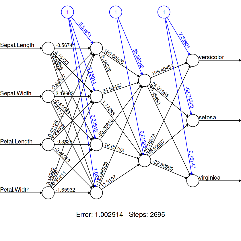
Model Evaluation
For the confusion matrix:
- We will predict categories using a test dataset.
- Create a list of category names.
- Create a prediction dataframe and replace numerical outputs with labels.
- Use tables to display ‘actual’ and ‘practiced’ values side by side.
pred <- predict(model, test_data)
labels <- c("setosa", "versicolor", "virginca")
prediction_label <- data.frame(max.col(pred)) %>%
mutate(pred=labels[max.col.pred.]) %>%
select(2) %>%
unlist()

table(test_data$Species, prediction_label)
We got almost perfect results. It seems that our model has wrongfully predicted three samples. We can improve the result by adding more neurons in each layer.
           prediction_label
            setosa versicolor virginica
  setosa          8          0        0
  versicolor      0         13        0
  virginica       0          3        6
To check the accuracy, we have to first convert actual categorical values into numerical ones and compare them with predicted values. As a result, we will receive a list of boolean values.
We can use the `sum` function to find the number of `TRUE` values and divide it by the total number of samples to get the accuracy.
check = as.numeric(test_data$Species) == max.col(pred)
accuracy = (sum(check)/nrow(test_data))*100
print(accuracy)
The model has predicted values with 90% accuracy.
90Note: the code source for this example is available on R workspace: Building Neural Network (NN) Models in R.
Convolutional Neural Network in R with Keras
In this example, we will use Keras and TensorFlow to build and train a Convolutional Neural Network model for the image classification task. For that, we will use the cifar10 image dataset consisting of 60,000 32x32 color images labeled over ten categories.
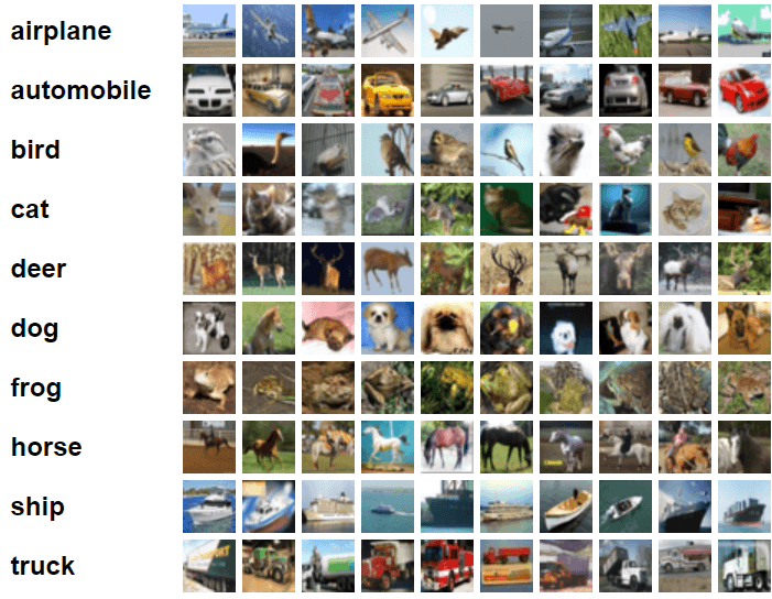
Image from CIFAR-10
Import essential R packages.
library(keras)
library(tensorflow)
Preparing the data
We will import Keras built-in dataset and split it into train and test sets.
c(c(x_train, y_train), c(x_test, y_test)) %<-% dataset_cifar10()Divide the train and test features by 255 to normalize the data.
x_train <- x_train / 255
x_test <-  x_test / 255
Building the model
Keras API provides us the flexibility to build fully customizable complex neural network architecture.
In our case, we will create multiple convolution layers, followed by the max pooling layer, dropout layer, dense layer, and output layer.
We are using ‘Leaky ReLU’ as an activation function for all layers except the output layer. For that, we are using ‘softmax’.
We need to set the input shape of the first 2D convolutional layer to the shape of image (32,32,3) of the training dataset.
model <- keras_model_sequential()%>%
  # Start with a hidden 2D convolutional layer
  layer_conv_2d(
    filter = 16, kernel_size = c(3,3), padding = "same",
    input_shape = c(32, 32, 3), activation = 'leaky_relu'
  ) %>%

  # 2nd hidden layer
  layer_conv_2d(filter = 32, kernel_size = c(3,3), activation = 'leaky_relu') %>%


  # Use max pooling
  layer_max_pooling_2d(pool_size = c(2,2)) %>%
  layer_dropout(0.25) %>%

  # 3rd and 4th hidden 2D convolutional layers
  layer_conv_2d(filter = 32, kernel_size = c(3,3), padding = "same", activation = 'leaky_relu') %>%

  layer_conv_2d(filter = 64, kernel_size = c(3,3), activation = 'leaky_relu') %>%

  # Use max pooling
  layer_max_pooling_2d(pool_size = c(2,2)) %>%
  layer_dropout(0.25) %>%

  # Flatten max filtered output into feature vector
  # and feed into dense layer
  layer_flatten() %>%
  layer_dense(256, activation = 'leaky_relu') %>%
  layer_dropout(0.5) %>%

  # Outputs from dense layer
  layer_dense(10, activation = 'softmax')
To view model architecture, we will use the `summary` function.
summary(model)We have two convolutional layers followed by a max pooling layer, two more convolutional layers, a max pooling layer, a flattened layer to max filtered output into vectors, and then two dense layers.
Model: "sequential"
________________________________________________________________________________
Layer (type)                        Output Shape                    Param #
================================================================================
conv2d_3 (Conv2D)                   (None, 32, 32, 16)              448
________________________________________________________________________________
conv2d_2 (Conv2D)                   (None, 30, 30, 32)              4640
________________________________________________________________________________
max_pooling2d_1 (MaxPooling2D)      (None, 15, 15, 32)              0
________________________________________________________________________________
dropout_2 (Dropout)                 (None, 15, 15, 32)              0
________________________________________________________________________________
conv2d_1 (Conv2D)                   (None, 15, 15, 32)              9248
________________________________________________________________________________
conv2d (Conv2D)                     (None, 13, 13, 64)              18496
________________________________________________________________________________
max_pooling2d (MaxPooling2D)        (None, 6, 6, 64)                0
________________________________________________________________________________
dropout_1 (Dropout)                 (None, 6, 6, 64)                0
________________________________________________________________________________
flatten (Flatten)                   (None, 2304)                    0
________________________________________________________________________________
dense_1 (Dense)                     (None, 256)                     590080
________________________________________________________________________________
dropout (Dropout)                   (None, 256)                     0
________________________________________________________________________________
dense (Dense)                       (None, 10)                      2570
================================================================================
Total params: 625,482
Trainable params: 625,482
Non-trainable params: 0
________________________________________________________________________________
Compiling the model
- We will be setting the learning rate using the schedule exponential decay function. It reduces the learning rate after 1500 steps by 0.98.
- Feed the learning rate object into the Adamax optimizer.
- Our loss function will be sparse categorical cross-entropy.
- Compile the model using loss and optimizer function, and performance metric.
learning_rate <- learning_rate_schedule_exponential_decay(
  initial_learning_rate = 5e-3,
  decay_rate = 0.96,
  decay_steps = 1500,
  staircase = TRUE
)
opt <- optimizer_adamax(learning_rate = learning_rate)

loss <- loss_sparse_categorical_crossentropy(from_logits = TRUE)


model %>% compile(
  loss = loss,
  optimizer = opt,
  metrics = "accuracy"
)
Training the model
We will fit our model and store the evaluation metric in `history`.
- We are going to train a model for 10 epochs and set the batch size to 32.
- Adding test dataset for validation.
- The `shuffle` argument will shuffle training data at the start of each epoch.
history <- model %>% fit(
  x_train, y_train,
  batch_size = 32,
  epochs = 10,
  validation_data = list(x_test, y_test),
  shuffle = TRUE
)
Evaluating the model
You can evaluate the model on a test dataset using the `evaluate` function, and it will return final loss and accuracy.
model %>% evaluate(x_test, y_test)Retraining the model on 50 epochs will improve model accuracy.
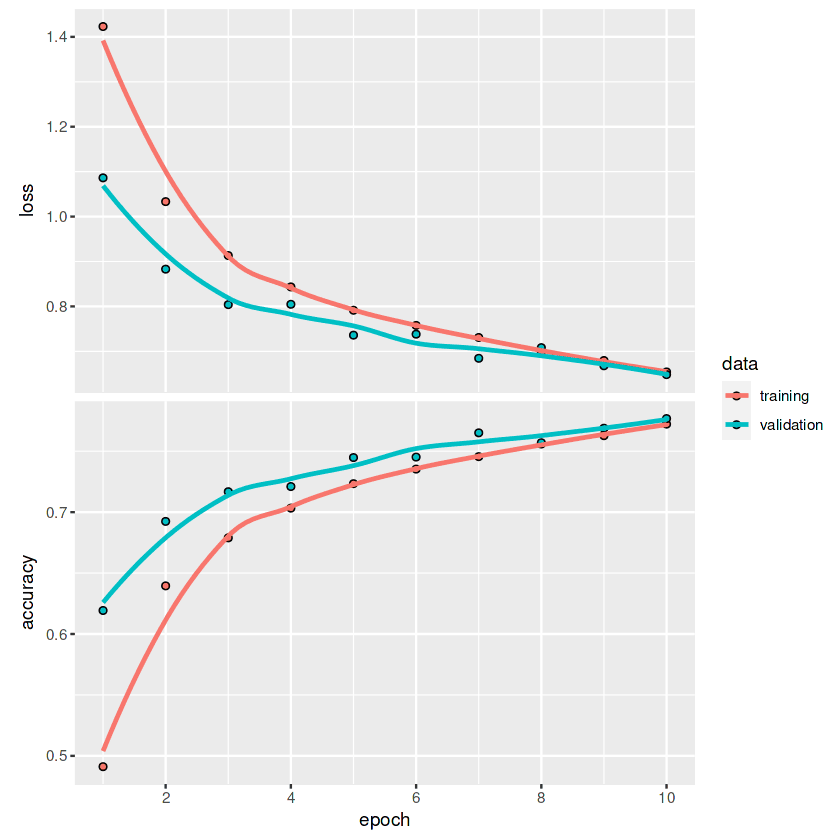
Loss 0.648191571235657 Accuracy 0.776799976825714To plot loss and accuracy line graphs for each epoch, we will use the `plot` function.
plot(history)By looking at the graph, we can observe that the line has not flattened yet. It means with higher epochs, we can improve the model metrics.
If you are interested in learning more about Keras API and how you can use it to build deep neural networks, check out keras: Deep Learning in R tutorial.
Applications of Neural Networks
We can find real-life neural network examples everywhere, from mobile applications to engineering. Due to the recent boom in language and large visual models, more companies are getting interested in implementing deep neural networks to increase profits and customer satisfaction.
In this section, we will learn about the top 10 applications of neural networks that are shaping the modern world.
1. Tabular Prediction
Simple neural networks are quite effective on large tabular data. We can use them for classification, clustering, and regression problems.
2. Stock Price Forecasting
A lot of companies are using LSTM, GRU, and RNN for financial forecasting. It allows them to make better decisions.
3. Medical Imaging
Breast cancer detection, anomaly detection, and image segmentation are some of the applications of Convolutional neural networks. Due to pre-trained transformers, we have seen advanced research in disease prevention and early detection of fatal illnesses.
4. E-commerce
Product recommendations, personalized experiences, and chatbots are some of the applications of neural networks used in E-commerce. These models are mainly used for clustering, natural language processing, and computer vision to improve customers' experience on the platform.
5. Generative Image
Due to the popularity of DALL·E 2 and stable diffusion, this space has become mainstream. Companies like Canva and Adobe have already implemented generative image capability to increase the number of users. Apart from mainstream hype, generative images are used in every industry to create synthetic data for improving the model's performance, stability, and biases.
6. Generative Text
ChatGPT, GPT-3, and GPT-NEO are the deep neural network models dominating the space. These models are used for programming assistance, chatbots, translation, question/answering, and more. It is everywhere, and companies are finding it easy to integrate it into their current systems.
7. Customer Service Chat Bot
DailoGPT and Blenderbot are popular conversational models enhancing your chatbot experience. They are adaptive and can be fine-tuned for a specific purpose. In the future, we won’t see long waiting times; these chatbots will be able to understand your problems and provide solutions in real time.
8. Robotics
Reinforcement learning and computer vision neural network models are playing a major role in transferring industries. For example, fully automated warehouse management, factories, and shopping experience.
9. Speech Recognition
Speech recognition, text-to-speech, and audio activity detection neural network models are used for speech assistance, automatic transcription, and enhanced communications applications.
10. Multimodal
Text to Image (DALLE-2), Image Text, Visual Question Answering, and feature extractions are some of the applications used in multimodal neural networks. In the future, you will see text-to-video with audio. You will be able to create a full movie by providing the script.
Conclusion
Keras and TensorFlow R package provide us with a full range of tools to create complex model architecture for specific tasks. You can load the dataset, perform pre-processing, build and optimize the model, and evaluate the model using a few lines of code. Furthermore, with Tensorflow, you can monitor your experiments, configure GPUs, and deploy the model to production.
In this tutorial, we have learned the basics of neural networks, the type of model architecture, and the application. Moreover, we have learned how to train a simple neural network using `neuralnet` and a convolutional neural network using `keras`. The tutorial covers the model building, compiling, training, and evaluation.
Learn more about Tensorflow and Keras API by taking Introduction to TensorFlow in R course. You will learn about tensorboard and other TensorFlow APIs, build deep neural networks, and improve model performance using regularization, dropout, and hyperparameter optimization.