Multiple Linear Regression in R: Tutorial With Examples

Regression methods are used in different industries to understand which variables impact a given topic of interest. 

For instance, Economists can use them to analyze the relationship between consumer spending and Gross Domestic Product (GDP) growth. Public health officials might want to understand the costs of individuals based on their historical information. In both cases, the focus is not on predicting individual scenarios but on getting an overview of the overall relationship.

In this article, we will start by providing a general understanding of regressions. Then, we will explain what makes simple and multiple linear regressions different before diving into the technical implementations and providing tools to help you understand and interpret the regression results.

What is Multiple Linear Regression?

Let’s first understand what a simple linear regression is before diving into multiple linear regression, which is just an extension of simple linear regression.

Simple linear regression

A simple linear regression aims to model the relationship between the magnitude of a single independent variable X and a dependent variable Y by trying to estimate exactly how much Y will change when X changes by a certain amount. 

• The independent variable X, also called the predictor, is the variable used to make the prediction. 
• The dependent variable Y, also known as the response, is the one we are trying to predict.

The “linear” aspect of linear regression is that we are trying to predict Y from X using the following “linear” equation. 

Y = b0 + b1X 

• b0 is the intercept of the regression line, corresponding to the predicted value when X is null. 
• b1 is the slope of the regression line.

So, what about multiple linear regression?

This is the use of linear regression with multiple variables, and the equation is:

Y = b0 + b1X1 + b2X2 + b3X3 + … + bnXn + e

• Y and b0 are the same as in the simple linear regression model. 
• b1X1 represents the regression coefficient (b1) on the first independent variable (X1). The same analysis applies to all the remaining regression coefficients and variables. 
• e is the model error (residuals), which defines how much variation is introduced in the model when estimating Y.

We might not always get a straight line for a multiple regression case. However, we can control the shape of the line by fitting a more appropriate model. 

These are some of the key elements computed by multiple linear regression to find the best fit line for each predictor.

• The estimated coefficients for each predictor. 
• r-square of the model, which corresponds to the proportion of variance explained by the model, and it measures the strength of the relationship between the model and the dependent variable Y on a convenient 0 to 100% scale. 
• the p-value and t-statistic for each regression coefficient in the model. These two metrics are considered to be the mirror of one another, and they measure the extent to which a given coefficient is statistically significant. The higher the t-statistic (which goes with the p-value near 0), the more significant the predictor is, meaning that this predictor should be kept in the model. On the other hand, a very low t-statistic (higher p-value) means that the predictor should be dropped.

The Multiple Linear Regression Assumptions

An important aspect when building a multiple linear regression model is to make sure that the following key assumptions are met.

• The residual values are normally distributed. This can be checked by either using a normal probability plot or a histogram.
• There must be a linear relationship between the dependent and the independent variables. This can be illustrated by scatterplots showing a linear or curvilinear relationship.
• Then, multicollinearity is another assumption, meaning that the independent variables are not highly correlated with each other. Multicollinearity makes it difficult to identify which variables better explain the dependent variable. This assumption is verified by computing a matrix of Pearson’s bivariate correlations among all the independent variables. If there is no collinearity in the data, then all the values should be less than 0.8. 
• The homoscedasticity assumes that the variance of the residual errors is similar across the value of each independent variable. One way of checking that is through a plot of the predicted values against the standardized residual values to see if the points are equally distributed across all the values of the independent variables.

In the next sections, we will cover some of these assumptions.

A Step-By-Step Guide to Multiple Linear Regression in R

In this section, we will dive into the technical implementation of a multiple linear regression model using the R programming language. 

We will use the customer churn data set from DataCamp’s workspace to estimate the customer value.

What do we mean by customer value? Basically, it determines how worth a product or service is to a customer, and we can calculate it as follows: 

Customer Value = Benefit — Cost. Where Benefit and Cost are, respectively, the benefit and cost of a product or a service. 

This value is higher if the company can offer consumers higher benefits and lower costs, or ideally, a combination of both.

This analysis could help the business identify the most promising targeting opportunity or next best action based on the value of a given customer.

Quick data exploration

Let’s have a quick overview of the data set so we can apply the relevant preprocessing before fitting the model.

churn_data = read_csv('data/customer_churn.csv', show_col_types = FALSE)
# Look at the first 6 observations
head(churn_data)
# Check the dimension
dim(churn_data)

First 6 rows of the data (Animation by Author)

From the previous results, we can observe that the data set has 3150 observations and 14 columns. 

However, based on the problem statement, we will not need the churn column because we are now dealing with a regression problem.

Before fitting the model, let’s preprocess the column names by replacing spaces in the column names with underscores to avoid writing the double quote around the variable names every time.

# Change the column names
names(churn_data) = gsub(" ", "_", names(churn_data))

head(churn_data)

First 6 rows after column names transformation (animation by author)

With this newly formatted data, we can fit it into the multiple regression framework using the lm() function in R as follows:

# Fit the multiple linear regression model
cust_value_model = lm(formula = Customer_Value ~ Call_Failure + 

                     Complaints + Subscription_Length + Charge_Amount +    

                     Seconds_of_Use +Frequency_of_use + Frequency_of_SMS +
                    Distinct_Called_Numbers + Age_Group + Tariff_Plan +
                    Status + Age,data = churn_data)

Let’s understand what we just did here.

The lm() function is in the following format: lm(formula = Y ~Sum(Xi), data = our_data)

• Y is the Customer_Value column because it is the one we are trying to estimate.
• Sum(Xi) represents the sum expression in the multiple linear regression equation. 
• our_data is the churn_data.

You can learn more from our Intermediate Regression in R course. 

An alternative to using R is the Intermediate Regression with statsmodels in Python. Both help you learn linear and logistic regression with multiple explanatory variables.

What Does the Multiple Linear Regression Model Tell Us?

Now that we have built the model, the next step is to check the assumptions and interpret the results. For simplicity, we will not cover all the aspects.

Distribution of the model residuals 

This can be shown in R using the hist() function.

# Get the model residuals
model_residuals = cust_value_model$residuals

# Plot the result
hist(model_residuals)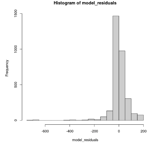

Model residuals distribution (Image by Author)

The histogram looks skewed to the left; hence we can not conclude the normality with enough confidence. Instead of the histogram, let’s look at the residuals along the normal Q-Q plot. If there is normality, then the values should follow a straight line.

# Plot the residuals
qqnorm(model_residuals)
# Plot the Q-Q line
qqline(model_residuals)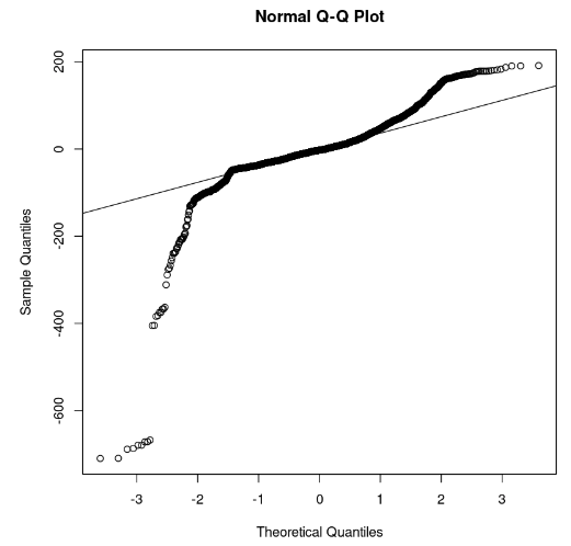

Q-Q plot and residuals (Image by Author)

From the plot, we can observe that a few portions of the residuals lie in a straight line. Then we can assume that the residuals of the model do not follow a normal distribution.  

Multicollinearity assumption check 

This is done through the following R code. But we have to remove the Customer_Value column beforehand.

# Install and load the ggcorrplot package
install.packages("ggcorrplot")
library(ggcorrplot)

# Remove the Customer Value column
reduced_data <- subset(churn_data, select = -Customer_Value)

# Compute correlation at 2 decimal places
corr_matrix = round(cor(reduced_data), 2)

# Compute and show the  result
ggcorrplot(corr_matrix, hc.order = TRUE, type = "lower",
          lab = TRUE)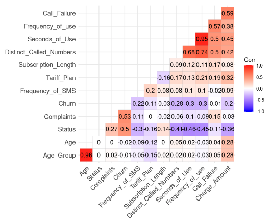

Correlation result from the data (Image by Author)

We can notice two strong correlations because their value is higher than 0.8. 

• Age and Age_Group: 0.96
• Frequency_of_Use and Second_of_Use: 0.95

This result makes sense because Age_Group is computed from Age. Also, the total number of seconds (Second_of_Use) is derived from the total number of calls (Frequency_of_Use). 

In this case, we can get rid of the Age_Group and Second_of_Use in the dataset. 

Let’s try to build a second model without those two variables.

second_model = lm(formula = Customer_Value ~ Call_Failure + Complaints +
                    Subscription_Length + Charge_Amount +
                    Frequency_of_use + Frequency_of_SMS +
                    Distinct_Called_Numbers + Tariff_Plan +
                    Status + Age,
                    data = churn_data)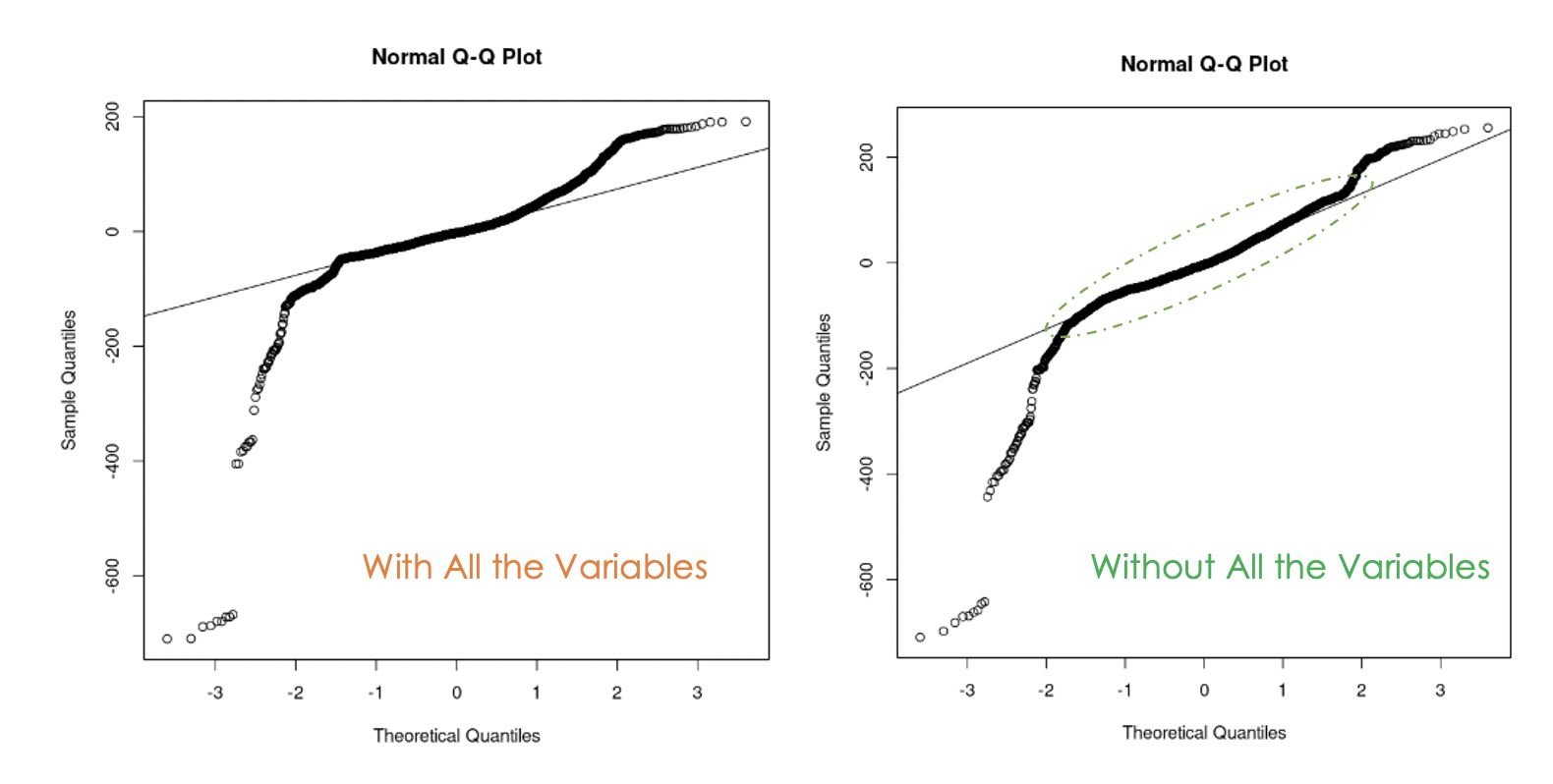

Q-Q plots of the first model (left) and the second model (right)

We can notice that getting rid of the multicollinearity in the data was helpful because, with the second model, more residual values are on the straight line compared to the first model.

How to Know Which of the Two Models is Better? 

One way of answering this question is to run an analysis of variance (ANOVA) test of the two models. It tests the null hypothesis (H0), where the variables that we removed previously have no significance, against the alternative hypothesis (H1) that those variables are significant. 

If the new model is an improvement of the original model, then we fail to reject H0. If that is not the case, it means that those variables were significant; hence we reject H0. 

Here is the general expression: anova(original_model, new_model)

# Anova test
anova(cust_value_model, second_model)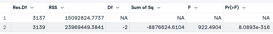

ANOVA test result (Image by Author)

From the ANOVA result, we observe that the p-value (8.0893e-316) is very small (less than 0.05), so we reject the null hypothesis, meaning that the second model is not an improvement of the first one. 

Another way of looking at the important variables in the model is through a significance test. 

A variable will be significant if its p-value is less than 0.05. This result can be generated by the summary() function. In addition to providing that information about the model it also renders the adjusted R-square, which evaluates the performance of models against each other.

# Print the result of the model
summary(cust_value_model)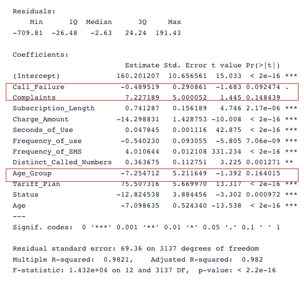

Summary Result for the original model with all the predictors (Image by Author)

We have two key sections in the table: Residuals and Coefficients. The Q-Q plots give the same information as the Residuals section. In the Coefficients section, Call_Failure, Complaints, and Age_Group are not considered to be significant by the model because their p-value is higher than 0.05. Keeping them does not provide any additional value to the model.

Applying the same analysis to the second model, we get this result:

summary(second_model)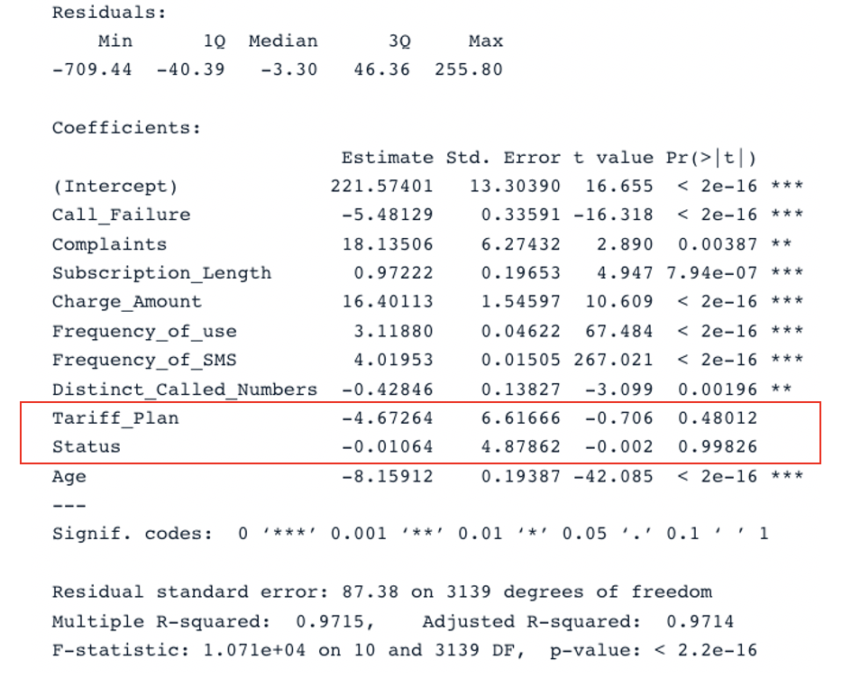

Summary Result for the second model with all the predictors (Image by Author)

The original model has an adjusted R-square of 0.98, which is higher than the second model’s adjusted R-square (0.97). This means that the original model with all the predictors is better than the second model.

Improve the multiple linear regression model

The logical next step of this analysis is to remove the non-significant variables and fit the model to see if the performance improves.

Another strategy for efficiently choosing relevant predictors is through the Akaike Information Criteria (AIC). 

It starts with all the features, then gradually drops the worst predictors one at a time until it finds the best model. The smaller the AIC score, the better the model. This can be done using the stepAIC() function.

Conclusion

This tutorial has covered the main aspects of multiple linear regressions and explored some strategies to build robust models. 

We hope this tutorial provides you with the relevant skills to get actionable insights from your data. You can try to improve these models by applying different approaches using the source code available from our workspace.