Multilayer Perceptrons in Machine Learning: A Comprehensive Guide

TL;DR

• A multilayer perceptron (MLP) is a feedforward neural network with one or more hidden layers that can learn non-linear patterns in data.
• MLPs consist of an input layer, hidden layers with nonlinear activation functions, and an output layer.
• Training uses backpropagation to compute gradients and stochastic gradient descent (SGD) to update weights iteratively.
• Data preparation is critical: clean, scale, and split your data before training an MLP.
• Start with a small architecture and increase complexity gradually, using regularization techniques to prevent overfitting.

Basics of Neural Networks

Neural networks or artificial neural networks are fundamental tools in machine learning, powering many state-of-the-art algorithms and applications across various domains, including computer vision, natural language processing, robotics, and more.

A neural network consists of interconnected nodes, called neurons, organized into layers. Each neuron receives input signals, performs a computation on them using an activation function, and produces an output signal that may be passed to other neurons in the network. An activation function determines the output of a neuron given its input. These functions introduce nonlinearity into the network, enabling it to learn complex patterns in data.

The network is typically organized into layers, starting with the input layer, where data is introduced. Followed by hidden layers where computations are performed and finally, the output layer where predictions or decisions are made.

Neurons in adjacent layers are connected by weighted connections, which transmit signals from one layer to the next. The strength of these connections, represented by weights, determines how much influence one neuron's output has on another neuron's input. During the training process, the network learns to adjust its weights based on examples provided in a training dataset. Additionally, each neuron typically has an associated bias, which allows the neuron to adjust its output threshold.

Neural networks are trained usingtechniques called feedforward propagation andbackpropagation. During feedforward propagation, input data is passed through the network layer by layer, with each layer performing a computation based on the inputs it receives and passing the result to the next layer.

Backpropagation is an algorithm used to train neural networks by iteratively adjusting the network's weights and biases in order to minimize the loss function. A loss function (also known as a cost function or objective function) is a measure of how well the model's predictions match the true target values in the training data. The loss function quantifies the difference between the predicted output of the model and the actual output, providing a signal that guides the optimization process during training.

The goal of training a neural network is to minimize this loss function by adjusting the weights and biases. The adjustments are guided by an optimization algorithm,such as gradient descent. We will revisitsome of these topics in more detail later on in this tutorial.

Types of Neural Networks

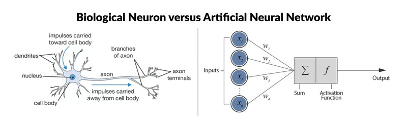
Biological neuron vs. artificial neural network (Source: ResearchGate)

The ANN depicted on the right of the image is a simple neural network called ‘perceptron’. It consists of a single layer, which is the input layer, with multiple neurons with their own weights; there are no hidden layers. The perceptron algorithm learns the weights for the input signals in order to draw a linear decision boundary.

However, to solve more complicated, non-linear problems related to image processing, computer vision, and natural language processing tasks, we work with deep neural networks.

Check out our Introduction to Deep Neural Networks tutorial to learn more about deep neural networks and how to construct one from scratch, utilizing TensorFlow and Keras in Python. If you would prefer to use the R language instead, our Building Neural Network (NN) Models in R has you covered.

There are several types of ANN, each designed for specific tasks and architectural requirements. Let's briefly discuss some of the most common types before diving deeper into MLPs next.

Feedforward Neural Networks (FNN)

These are the simplest form of ANNs, where information flows in one direction, from input to output. There are no cycles or loops in the network architecture. Multilayer perceptrons (MLP) are a type of feedforward neural network.

Recurrent Neural Networks (RNN)

In RNNs, connections between nodes form directed cycles, allowing information to persist over time. This makes them suitable for tasks involving sequential data, such as time series prediction, natural language processing, and speech recognition.

Convolutional Neural Networks (CNN)

CNNs are designed to effectively process grid-like data, such as images. They consist of layers of convolutional filters that learn hierarchical representations of features within the input data. CNNs are widely used in tasks like image classification, object detection, and image segmentation.

Long Short-Term Memory Networks (LSTM) and Gated Recurrent Units (GRU)

These are specialized types of recurrent neural networks designed to address the vanishing gradient problem in traditional RNN. LSTMs and GRUs incorporate gated mechanisms to better capture long-range dependencies in sequential data, making them particularly effective for tasks like speech recognition, machine translation, and sentiment analysis.

Autoencoder

It is designed for unsupervised learning and consists of an encoder network that compresses the input data into a lower-dimensional latent space, and a decoder network that reconstructs the original input from the latent representation. Autoencoders are often used for dimensionality reduction, data denoising, and generative modeling.

Generative Adversarial Networks (GAN)

GANs consist of two neural networks, a generator and a discriminator, trained simultaneously in a competitive setting. The generator learns to generate synthetic data samples that are indistinguishable from real data, while the discriminator learns to distinguish between real and fake samples. GANs have been widely used for generating realistic images, videos, and other types of data.

What Is a Multilayer Perceptron (MLP)?

A multilayer perceptron is a type of feedforward neural network consisting of fully connected neurons with a nonlinear kind of activation function. It is widely used to distinguish data that is not linearly separable.

Components of an MLP

MLPs have been widely used in various fields, including image recognition, natural language processing, and speech recognition, among others. Their flexibility in architecture and ability to approximate any function under certain conditions make them a fundamental building block in deep learning and neural network research. Let's take a deeper dive into some of its key concepts.

Input layer

The input layer consists of nodes or neurons that receive the initial input data. Each neuron represents a feature or dimension of the input data. The number of neurons in the input layer is determined by the dimensionality of the input data.

Hidden layer

Between the input and output layers, there can be one or more layers of neurons. Each neuron in a hidden layer receives inputs from all neurons in the previous layer (either the input layer or another hidden layer) and produces an output that is passed to the next layer. The number of hidden layers and the number of neurons in each hidden layer are hyperparameters that need to be determined during the model design phase.

Output layer

This layer consists of neurons that produce the final output of the network. The number of neurons in the output layer depends on the nature of the task. In binary classification, there may be either one or two neurons depending on the activation function and representing the probability of belonging to one class; while in multi-class classification tasks, there can be multiple neurons in the output layer.

Weights

Neurons in adjacent layers are fully connected to each other. Each connection has an associated weight, which determines the strength of the connection. These weights are learned during the training process.

Bias neurons

In addition to the input and hidden neurons, each layer (except the input layer) usually includes a bias neuron that provides a constant input to the neurons in the next layer. Bias neurons have their own weight associated with each connection, which is also learned during training.

The bias neuron effectively shifts the activation function of the neurons in the subsequent layer, allowing the network to learn an offset or bias in the decision boundary. By adjusting the weights connected to the bias neuron, the MLP can learn to control the threshold for activation and better fit the training data.

Note: It is important to note that in the context of MLPs, bias can refer to two related but distinct concepts: bias as a general term in machine learning and the bias neuron (defined above). In general machine learning, bias refers to the error introduced by approximating a real-world problem with a simplified model. Bias measures how well the model can capture the underlying patterns in the data. A high bias indicates that the model is too simplistic and may underfit the data, while a low bias suggests that the model is capturing the underlying patterns well.

Activation function

Typically, each neuron in the hidden layers and the output layer applies an activation function to its weighted sum of inputs. Common activation functions include sigmoid, tanh, ReLU (Rectified Linear Unit), and softmax. These functions introduce nonlinearity into the network, allowing it to learn complex patterns in the data.

Feedforward and Backpropagation

MLPs are trained using the backpropagation algorithm, which computes gradients of a loss function with respect to the model's parameters and updates the parameters iteratively to minimize the loss.

How a Multilayer Perceptron Works: Layer by Layer

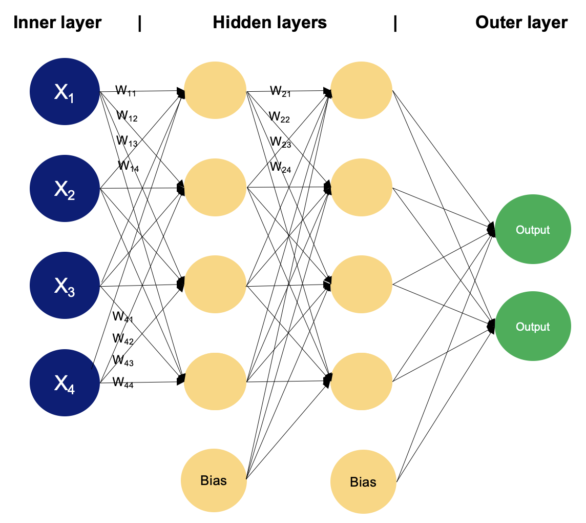
Example of an MLP with two hidden layers. Image by Author

In a multilayer perceptron, neurons process information in a step-by-step manner, performing computations that involve weighted sums and nonlinear transformations. Let's walk layer by layer to see the magic that goes within.

Input layer

• The input layer of an MLP receives input data, which could be features extracted from the input samples in a dataset. Each neuron in the input layer represents one feature.
• Neurons in the input layer do not perform any computations; they simply pass the input values to the neurons in the first hidden layer.

Hidden layers

• The hidden layers of an MLP consist of interconnected neurons that perform computations on the input data.
• Each neuron in a hidden layer receives input from all neurons in the previous layer. The inputs are multiplied by corresponding weights, denoted as w. The weights determine how much influence the input from one neuron has on the output of another.
• In addition to weights, each neuron in the hidden layer has an associated bias, denoted as b. The bias provides an additional input to the neuron, allowing it to adjust its output threshold. Like weights, biases are learned during training.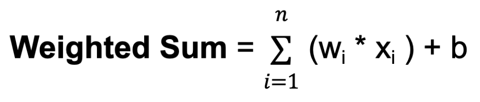
• For each neuron in a hidden layer or the output layer, the weighted sum of its inputs is computed. This involves multiplying each input by its corresponding weight, summing up these products, and adding the bias:

Where n is the total number of input connections, wi is the weight for the i-th input, and xi is the i-th input value.

• The weighted sum is then passed through an activation function, denoted as f. The activation function introduces nonlinearity into the network, allowing it to learn and represent complex relationships in the data. The activation function determines the output range of the neuron and its behavior in response to different input values. The choice of activation function depends on the nature of the task and the desired properties of the network.

Output layer

• The output layer of an MLP produces the final predictions or outputs of the network. The number of neurons in the output layer depends on the task being performed (e.g., binary classification, multi-class classification, regression).
• Each neuron in the output layer receives input from the neurons in the last hidden layer and applies an activation function. This activation function is usually different from those used in the hidden layers and produces the final output value or prediction.

During the training process, the network learns to adjust the weights associated with each neuron's inputs to minimize the discrepancy between the predicted outputs and the true target values in the training data. By adjusting the weights and learning the appropriate activation functions, the network learns to approximate complex patterns and relationships in the data, enabling it to make accurate predictions on new, unseen samples.

This adjustment is guided by an optimization algorithm,such as stochastic gradient descent (SGD), which computesthe gradients of a loss function with respect to the weights and updates the weights iteratively.

Let’s take a closer look at how SGD works.

Stochastic Gradient Descent (SGD)

1. Initialization: SGD starts with an initial set of model parameters (weights and biases) randomly or using some predefined method.
2. Iterative optimization: The aim of this step is to find the minimum of a loss function, by iteratively moving in the direction of the steepest decrease in the function's value. For each iteration (or epoch) of training:
   • Shuffle the training data to ensure that the model doesn't learn from the same patterns in the same order every time.
   • Split the training data into mini-batches (small subsets of data).
   • For each mini-batch:
     • Compute the gradient of the loss function with respect to the model parameters using only the data points in the mini-batch. This gradient estimation is a stochastic approximation of the true gradient.
     • Update the model parameters by taking a step in the opposite direction of the gradient, scaled by the learning rate:

θₜ₊₁ = θₜ − η ∇J(θₜ)

Where:

• θₜ represents the model parameters (e.g., weights and biases) at iteration t

• ∇J(θₜ) is the gradient of the loss function J with respect to the parameters at iteration t

• η (eta) is the learning rate, which controls the step size during optimization

3. Direction of descent: The gradient of the loss function indicates the direction of the steepest ascent. To minimize the loss function, gradient descent moves in the opposite direction, towards the steepest descent.
4. Learning rate: The step size taken in each iteration of gradient descent is determined by a parameter calledthe learning rate, denoted above asn. This parameter controls the size of the steps taken towards the minimum. If the learning rate is too small, convergence may be slow; if it is too large, the algorithm may oscillate or diverge.
5. Convergence: Repeat the process for a fixed number of iterations or until a convergence criterion is met (e.g., the change in loss function is below a certain threshold).

Stochastic gradient descent updates the model parameters more frequently using smaller subsets of data, making it computationally efficient, especially for large datasets. The randomness introduced by SGD can have a regularization effect, preventing the model from overfitting to the training data. It is also well-suited for online learning scenarios where new data becomes available incrementally, as it can update the model quickly with each new data point or mini-batch.

However, SGD can also have some challenges, such as increased noise due to the stochastic nature of the gradient estimation and the need to tune hyperparameters like the learning rate. Various extensions and adaptations of SGD, such as mini-batch stochastic gradient descent, momentum, and adaptive learning rate methods like AdaGrad, RMSProp, and Adam, have been developed to address these challenges and improve convergence and performance.

You have seen the working of the multilayer perceptron layers and learned about stochastic gradient descent; to put it all together, there is one last topic to dive into: backpropagation.

Backpropagation

Backpropagation is short for “backward propagation of errors.” In the context of backpropagation, SGD involves updating the network's parameters iteratively based on the gradients computed during each batch of training data. Instead of computing the gradients using the entire training dataset (which can be computationally expensive for large datasets), SGD computes the gradients using small random subsets of the data called mini-batches. Here’s an overview of how backpropagation algorithm works:

1. Forward pass: During the forward pass, input data is fed into the neural network, and the network's output is computed layer by layer. Each neuron computes a weighted sum of its inputs, applies an activation function to the result, and passes the output to the neurons in the next layer.
2. Loss computation: After the forward pass, the network's output is compared to the true target values, and a loss function is computed to measure the discrepancy between the predicted output and the actual output.
3. Backward pass (gradient calculation): In the backward pass, the gradients of the loss function with respect to the network's parameters (weights and biases) are computed using the chain rule of calculus. The gradients represent the rate of change of the loss function with respect to each parameter and provide information about how to adjust the parameters to decrease the loss.
4. Parameter update: Once the gradients have been computed, the network's parameters are updated in the opposite direction of the gradients in order to minimize the loss function. This update is typically performed using an optimization algorithm such as stochastic gradient descent (SGD), that we discussed earlier.
5. Iterative process: Steps 1-4 are repeated iteratively for a fixed number of epochs or until convergence criteria are met. During each iteration, the network's parameters are adjusted based on the gradients computed in the backward pass, gradually reducing the loss and improving the model's performance.

Data Preparation for MLPs

Preparing data for training an MLP involves cleaning, preprocessing, scaling, splitting, formatting, and maybe even augmenting the data. Based on the activation functions used and the scale of the input features, the data might need to bestandardized or normalized. Experimentingwith different preprocessing techniques and evaluating their impact on model performance is often necessary to determine the most suitable approach for a particular dataset and task.

• Data cleaning and preprocessing
  • Handle missing values: Remove or impute missing values in the dataset.
  • Encode categorical variables: Convert categorical variables into numerical representations, such as one-hot encoding.
• Feature scaling
  • Standardization or normalization: Rescale the features to a similar scale to ensure that the optimization process converges efficiently.
    • Standardization (Z-score normalization): Subtract the mean and divide by the standard deviation of each feature. It centers the data around zero and scales it to have unit variance.
    • Normalization (Min-Max scaling): Scale the features to a fixed range, typically between 0 and 1, by subtracting the minimum value and dividing by the range (max-min).

To learn more about feature scaling,check out Datacamp’s Feature Engineering for Machine Learning in Python course.

• Train-validation-test split
  • Split the dataset into training, validation, and test sets. The training set is used to train the model, the validation set is used to tune hyperparameters and monitor model performance, and the test set is used to evaluate the final model's performance on unseen data.
• Data formatting
  • Ensure that the data is in the appropriate format for training. This may involve reshaping the data or converting it to the required data type (e.g., converting categorical variables to numeric).
• Optional data augmentation
  • For tasks such as image classification, data augmentation techniques such as rotation, flipping, and scaling may be applied to increase the diversity of the training data and improve model generalization.
• Normalization and activation functions
  • The choice between standardization and normalization may depend on the activation functions used in the MLP. Activation functions like sigmoid and tanh are sensitive to the scale of the input data and may benefit from standardization. On the other hand, activation functions like ReLU are less sensitive to the scale and may not require standardization.

Implementation Tips and Best Practices

Implementing a MLP involves several steps, from data preprocessing to model training and evaluation. Selecting the number of layers and neurons for a MLP involves balancing model complexity, training time, and generalization performance. There is no one-size-fits-all answer, as the optimal architecture depends on factors such as the complexity of the task, the amount of available data, and computational resources. However, here are some general guidelines to consider when implementing MLP:

1. Model architecture

• Begin with a simple architecture and gradually increase complexity as needed. Start with a single hidden layer and a small number of neurons, and then experiment with adding more layers and neurons if necessary.

2. Task complexity

• For simple tasks with relatively low complexity, such as binary classification or regression on small datasets, a shallow architecture with fewer layers and neurons may suffice.
• For more complex tasks, such as multi-class classification or regression on high-dimensional data, deeper architectures with more layers and neurons may be necessary to capture intricate patterns in the data.

3. Data preprocessing

• Clean and preprocess your data, including handling missing values, encoding categorical variables, and scaling numerical features.
• Split your data into training, validation, and test sets to evaluate the model's performance.

4. Initialization

• Initialize the weights and biases of your MLP appropriately. Common initialization techniques include random initialization with small weights or using techniques like Xavier or He initialization.

5. Experimentation

• Ultimately, the best approach is to experiment with different architectures, varying the number of layers and neurons, and evaluate their performance empirically.
• Use techniques such as cross-validation and hyperparameter tuning to systematically explore different architectures and find the one that performs best on the task at hand.

6. Training

• Train your MLP using the training data and monitor its performance on the validation set.
• Experiment with different batch sizes, number of epochs, and other hyperparameters to find the optimal training settings.
• Visualize training progress using metrics such as loss and accuracy to diagnose issues and track convergence.

7. Optimization algorithm

• Experiment with different learning rates and consider using techniques like learning rate schedules or adaptive learning rates.

8. Avoid overfitting

• Be cautious not to overfit the model to the training data by introducing unnecessary complexity.
• Use techniques such as regularization (e.g., L1, L2 regularization), dropout, and early stoppingto prevent overfitting and improve generalization performance.
• Tune the regularization strength based on the model's performance on the validation set.

9. Model evaluation

• Monitor the model's performance on a separate validation set during training to assess how changes in architecture affect performance.
• Evaluate the trained model on the test set to assess its generalization performance.
• Use metrics such as accuracy, loss, and validation error to evaluate the model's performance and guide architectural decisions.

10. Iterate and experiment

• Experiment with different architectures, hyperparameters, and optimization strategies to improve the model's performance.
• Iterate on your implementation based on insights gained from training and evaluation results.

Advantages and Limitations of MLPs

Before choosing an MLP for your project, it helps to understand where they excel and where other architectures may be a better fit.

Advantages

• Universal approximation: MLPs can approximate any continuous function given enough neurons and layers, making them highly flexible for a wide range of tasks.
• Non-linear modeling: Unlike single-layer perceptrons, MLPs handle non-linearly separable data through their hidden layers and nonlinear activation functions.
• Versatility: MLPs work well for classification, regression, and pattern recognition across domains like finance, healthcare, and natural language processing.
• Straightforward implementation: Libraries like Keras, PyTorch, and scikit-learn provide ready-to-use MLP implementations with minimal setup.

Limitations

• Not ideal for spatial or sequential data: For images, CNNs outperform MLPs by exploiting spatial structure. For sequences, RNNs and LSTMs capture temporal dependencies better.
• Prone to overfitting: With many parameters, MLPs can memorize training data. Techniques like regularization, dropout, and early stopping help mitigate this.
• Computationally expensive: Fully connected layers scale poorly as input dimensionality increases, requiring more parameters and training time than architectures like CNNs.
• Sensitive to feature scaling: MLPs require properly scaled input features for efficient convergence during training.
• Black-box nature: Interpreting what an MLP has learned is more challenging compared to tree-based models or linear methods.

Conclusion

Multilayer perceptrons represent a fundamental and versatile class of artificial neural networks that have significantly contributed to the advancement of machine learning and artificial intelligence. Through their interconnected layers of neurons and nonlinear activation functions, MLPs are capable of learning complex patterns and relationships in data, making them well-suited for a wide range of tasks. The history of MLPs reflects a journey of exploration, discovery, and innovation, from the early perceptron models to the modern deep learning architectures that power many state-of-the-art systems today.

In this article, you’ve learned the basics of artificial neural networks, focused on multilayer perceptrons, learned about stochastic gradient descent and backpropagation. If you are interested in getting hands-on experience and using deep learning techniques to solve real-world challenges, such as predicting housing prices, building neural networks to model images and text - we highly recommend following our Keras toolbox track.

Working with Keras, you’ll learn about neural networks, deep learning model workflows, and how to optimize your models.Datacamp also has a Keras cheat sheet that can come in handy!