Course
Imagine being in a zoo trying to recognize if a given animal is a cheetah or a leopard. As a human, your brain can effortlessly analyze body and facial features to come to a valid conclusion. In the same way, Convolutional Neural Networks (CNNs) can be trained to perform the same recognition task, no matter how complex the patterns are. This makes them powerful in the field of computer vision.
This conceptual CNN tutorial will start by providing an overview of what CNNs are and their importance in machine learning. Then it will walk you through a step-by-step implementation of CNN in TensorFlow Framework 2.
What is a CNN?
A Convolutional Neural Network (CNN or ConvNet) is a deep learning algorithm specifically designed for any task where object recognition is crucial such as image classification, detection, and segmentation. Many real-life applications, such as self-driving cars, surveillance cameras, and more, use CNNs.
The importance of CNNs
These are several reasons why CNNs are important, as highlighted below:
- Unlike traditional machine learning models like SVM and decision trees that require manual feature extractions, CNNs can perform automatic feature extraction at scale, making them efficient.
- The convolutions layers make CNNs translation invariant, meaning they can recognize patterns from data and extract features regardless of their position, whether the image is rotated, scaled, or shifted.
- Multiple pre-trained CNN models such as VGG-16, ResNet50, Inceptionv3, and EfficientNet are proved to have reached state-of-the-art results and can be fine-tuned on news tasks using a relatively small amount of data.
- CNNs can also be used for non-image classification problems and are not limited to natural language processing, time series analysis, and speech recognition.
Architecture of a CNN
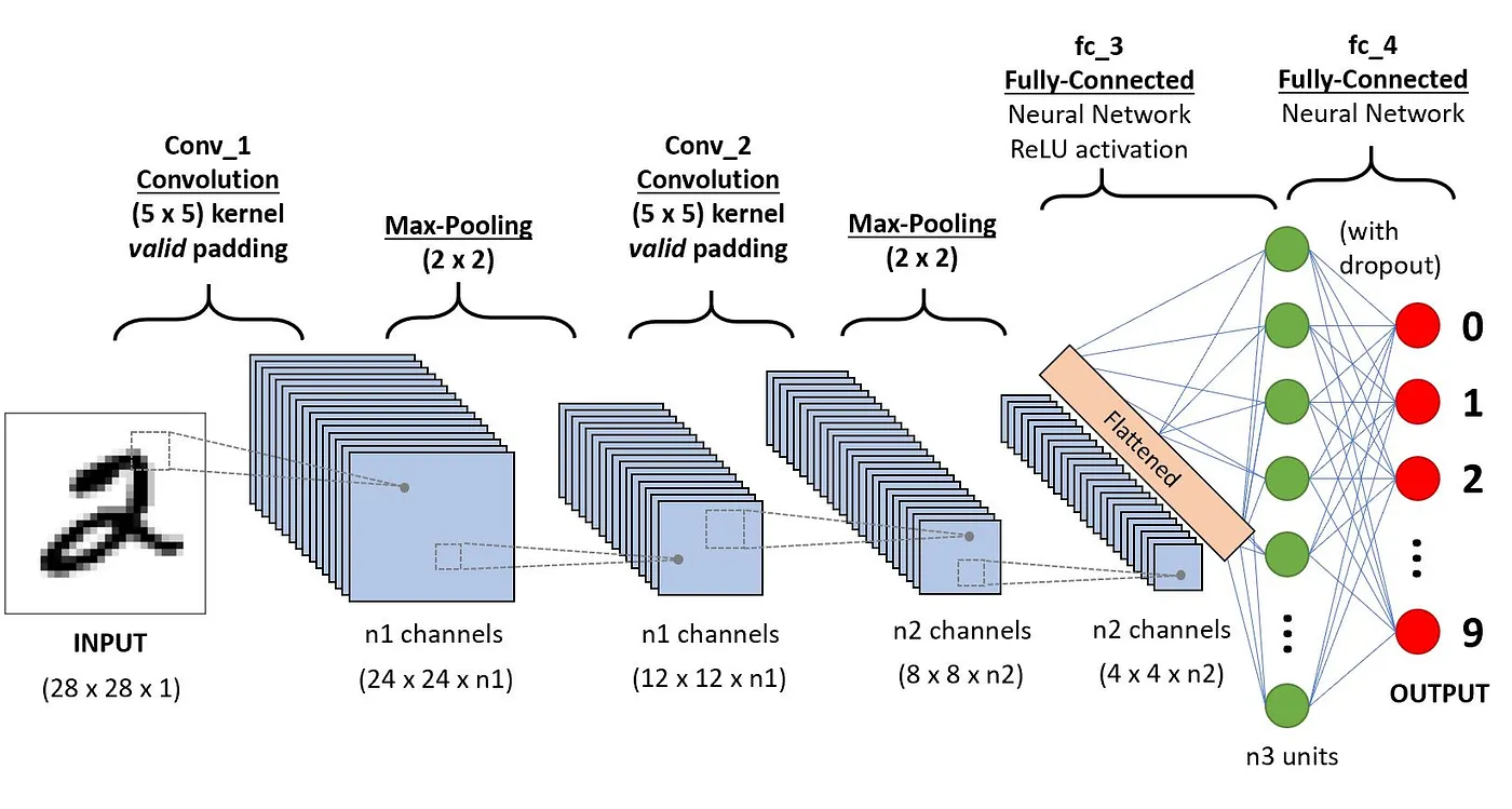
CNNs’ architecture tries to mimic the structure of neurons in the human visual system composed of multiple layers, where each one is responsible for detecting a specific feature in the data. As illustrated in the image below, the typical CNN is made of a combination of four main layers:
- Convolutional layers
- Rectified Linear Unit (ReLU for short)
- Pooling layers
- Fully connected layers
Let’s understand how each of these layers works using the following example of classification of the handwritten digit.
Convolution layers
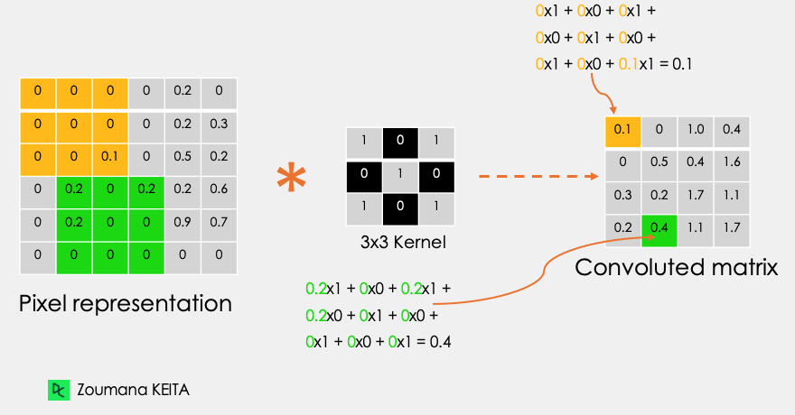
This is the first building block of a CNN. As the name suggests, the main mathematical task performed is called convolution, which is the application of a sliding window function to a matrix of pixels representing an image. The sliding function applied to the matrix is called kernel or filter, and both can be used interchangeably.
In the convolution layer, several filters of equal size are applied, and each filter is used to recognize a specific pattern from the image, such as the curving of the digits, the edges, the whole shape of the digits, and more.
Let’s consider this 32x32 grayscale image of a handwritten digit. The values in the matrix are given for illustration purposes.
![]()
Also, let’s consider the kernel used for the convolution. It is a matrix with a dimension of 3x3. The weights of each element of the kernel is represented in the grid. Zero weights are represented in the black grids and ones in the white grid.
Do we have to manually find these weights?
In real life, the weights of the kernels are determined during the training process of the neural network.
Using these two matrices, we can perform the convolution operation by taking applying the dot product, and work as follows:
- Apply the kernel matrix from the top-left corner to the right.
- Perform element-wise multiplication.
- Sum the values of the products.
- The resulting value corresponds to the first value (top-left corner) in the convoluted matrix.
- Move the kernel down with respect to the size of the sliding window.
- Repeat from step 1 to 5 until the image matrix is fully covered.
The dimension of the convoluted matrix depends on the size of the sliding window. The higher the sliding window, the smaller the dimension.
Another name associated with the kernel in the literature is feature detector because the weights can be fine-tuned to detect specific features in the input image.
For instance:
- Averaging neighboring pixels kernel can be used to blur the input image.
- Subtracting neighboring kernel is used to perform edge detection.
The more convolution layers the network has, the better the layer is at detecting more abstract features.
Activation function
A ReLU activation function is applied after each convolution operation. This function helps the network learn non-linear relationships between the features in the image, hence making the network more robust for identifying different patterns. It also helps to mitigate the vanishing gradient problems.
Pooling layer
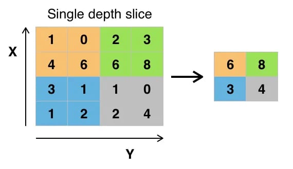
The goal of the pooling layer is to pull the most significant features from the convoluted matrix. This is done by applying some aggregation operations, which reduces the dimension of the feature map (convoluted matrix), hence reducing the memory used while training the network. Pooling is also relevant for mitigating overfitting.
The most common aggregation functions that can be applied are:
- Max pooling which is the maximum value of the feature map
- Sum pooling corresponds to the sum of all the values of the feature map
- Average pooling is the average of all the values.
Below is an illustration of each of the previous example:
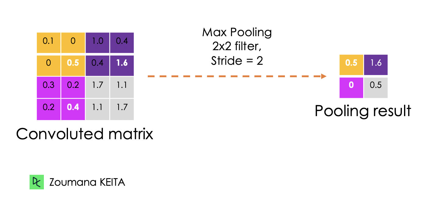
Also, the dimension of the feature map becomes smaller as the polling function is applied.
The last pooling layer flattens its feature map so that it can be processed by the fully connected layer.
Fully connected layers
These layers are in the last layer of the convolutional neural network, and their inputs correspond to the flattened one-dimensional matrix generated by the last pooling layer. ReLU activations functions are applied to them for non-linearity.
Finally, a softmax prediction layer is used to generate probability values for each of the possible output labels, and the final label predicted is the one with the highest probability score.
Dropout
Dropout is a regularization technic applied to improve the generalization capability of the neural networks with a large number of parameters. It consists of randomly dropping some neurons during the training process, which forces the remaining neurons to learn new features from the input data.
Since the technical implementation will be performed using TensorFlow 2, the next section aims to provide a complete overview of different components of this framework to efficiently build deep learning models.
What is the TensorFlow Framework?
Google developed TensorFlow in November 2015. They define it to be an open-source machine learning framework for everyone for several reasons.
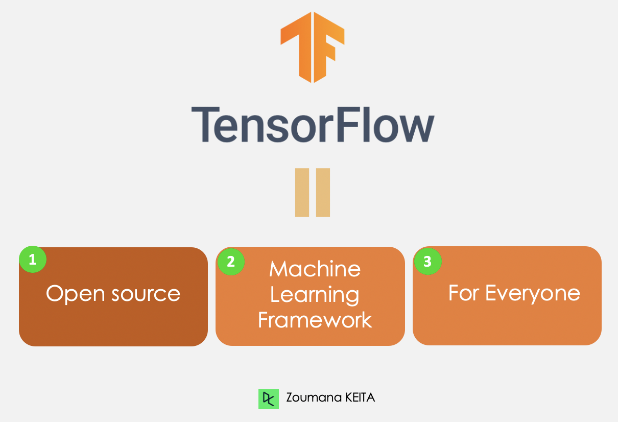
- Open-source: released under the Apache 2.0 open-source license. This allows researchers, organizations, and developers to make their contribution to the library by building upon it without any restrictions.
- Machine learning framework: meaning that it has a set of libraries and tools that support the building process of machine learning models.
- For everyone: Using TensorFlow makes the implementation of machine learning models easier through common programming languages like Python. Furthermore, built-in libraries such as Keras make it even easier to create robust deep learning models.
All these functionalities make Tensorflow a good candidate for building neural networks.
Furthermore, installing Tensorflow 2 is straightforward and can be performed as follows using the Python package manager pip as explained in the official documentation.
After the installation, we can see that the version being used is the 2.9.1
import tensorflow as tf
print("TensorFlow version:", tf.__version__)
Now, let’s further explore the main components for creating those networks.
What are Tensors?
We mainly deal with high-dimensional data when building machine learning and deep learning models. Tensors are multi-dimensional arrays with a uniform type used to represent different features of the data.
Below is the graphical representation of the different types of dimensions of tensors.
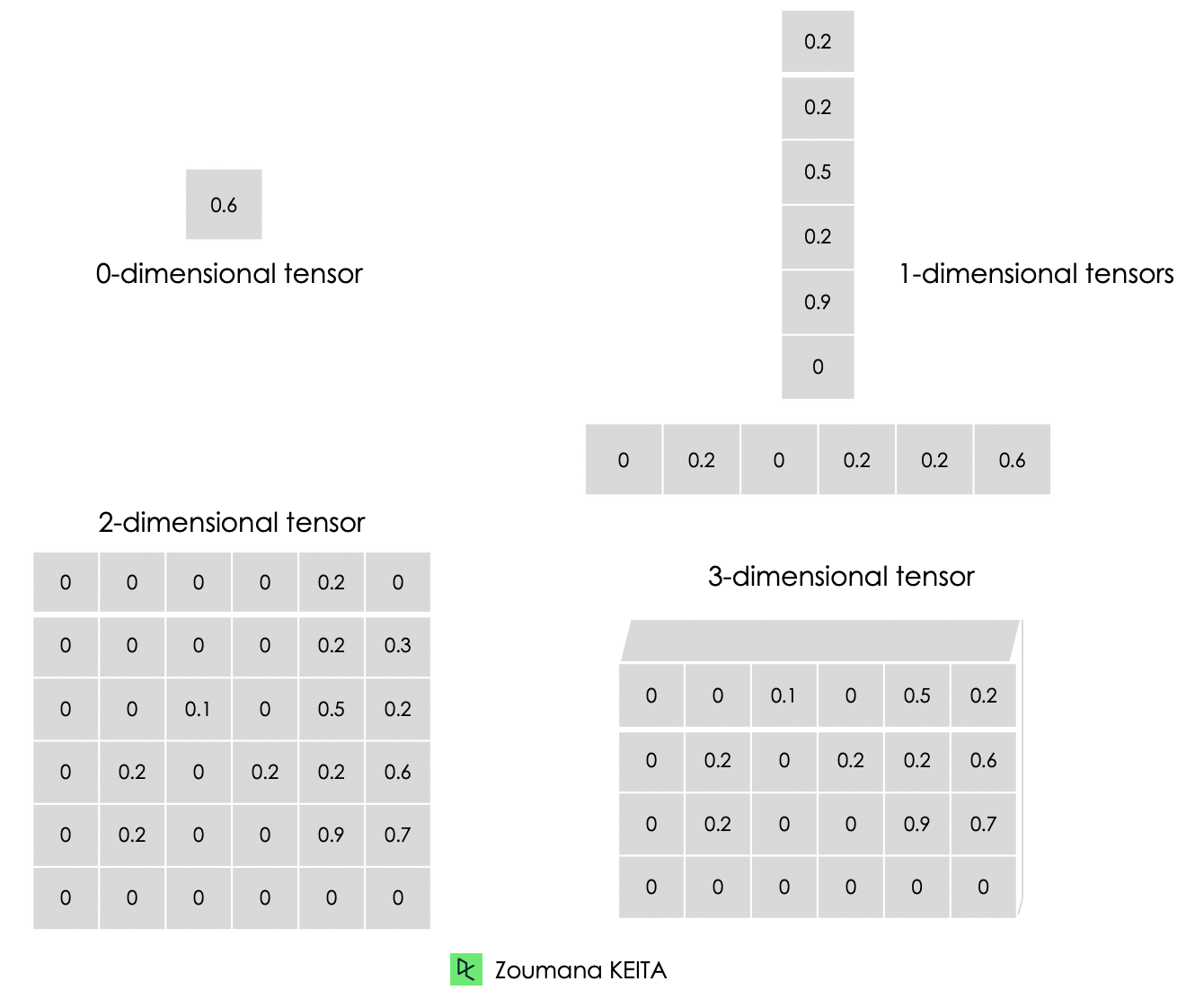
- A 0-dimensional tensor contains a single value.
- A 1-dimensional tensor, also known as “rank-1” tensor is list of values.
- A 2-dimensional tensor is a “rank-2” tensor.
- Finally, we can have a N-dimensional tensor, where N represents the number of dimensions within the tensor. In the previous cases, N is respectively 0, 1 and 2.
Below is an illustration of a zero to a 3-dimensional tensor. Each tensor is created using the constant() function from TensorFlow.
# Zero dimensional tensor
zero_dim_tensor = tf.constant(20)
print(zero_dim_tensor)

# One dimensional tensor
one_dim_tensor = tf.constant([12, 20, 53, 26, 11, 56])
print(one_dim_tensor)

# Two dimensional tensor
two_dim_array = [[3, 6, 7, 5],
             	[9, 2, 3, 4],
             	[7, 1, 10,6],
             	[0, 8, 11,2]]

two_dim_tensor = tf.constant(two_dim_array)
print(two_dim_tensor)
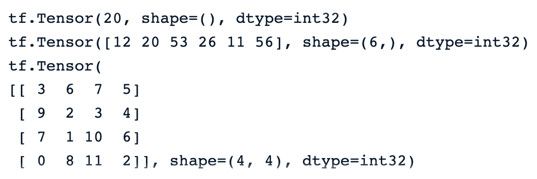
A successful execution of the previous code should generate the outputs below, and we can notice the keyword “tf.Tensor” to mean that the result is a tensor. It has three parameters:
- The actual value of the tensor.
- The shape() of the tensor, which is 0, 6 by 1, and 4 by 4, respectively for the first, second, and third tensors.
- The data type represented by the dtype attribute, and all the tensors are int32.
Our Tensorflow Tutorial for Beginners provides a complete overview of TensorFlow and teaches how to build and train models.
Tensors vs Matrices: Differences
Many people confuse tensors with matrices. Even though these two objects look similar, they have completely different properties. This section provides a better understanding of the difference between matrices and tensors.
- We can think of a matrice as a tensor with only two dimensions.
- Tensors, on the other hand, is a more general format that can have any number of dimensions.
As opposed to matrices, tensors are more suitable for deep learning problems for the following reasons:
- They can deal with any number of dimensions, which makes them a better fit for multi-dimensional data.
- Tensors’ ability to be compatible with a wide range of data types, shapes, and dimensions makes them more versatile than matrices.
- Tensorflow provides GPU and TPU support to speed up computations. Using tensors, machine learning engineers can automatically take advantage of these benefits.
- Tensors natively support broadcasting, which consists of making arithmetic operations between tensors of different shapes, which is not always possible when dealing with matrices.
TensorFlow: Constants, Variables, and Placeholders
Constants are not the only types of tensors. There are also variables and placeholders, which are all building blocks of a computational graph.
A computational graph is basically and a representation of a sequence of operations and the flow of data between them.
Now, let’s understand the difference between these types of tensors.
Constants
Constants are tensors whose values do not change during the execution of the computational graph. They are created using the tf.constant() function and are mainly used to store fixed parameters that do not require any change during the model training.
Variables
Variables are tensors whose value can be changed during the execution of the computational graph and they are created using the tf.Variable() function. For instance, in the case of neural networks, weights, and biases can be defined as variables since they need to be updated during the training process.
Placeholders
These were used in the first version of Tensorflow as empty containers that do not have specific values. They are just used to reverse a spot for data to be used in the future. This gives the users the freedom to use different datasets and batch sizes during model training and validation.
In Tensorflow version 2, placeholders have been replaced by the tf.function() function, which is a more Pythonic and dynamic approach to feeding data into the computational graph.
CNN Step-by-Step Implementation
Let’s put everything we have learned previously into practice. This section will illustrate the end-to-end implementation of a convolutional neural network in TensorFlow applied to the CIFAR-10 dataset, which is a built-in dataset with the following properties:
- It contains 60.000 32 by 32 color images
- The dataset has 10 different classes
- Each class has 6000 images
- There are overall 50.000 training images
- And overall 10.000 testing images
The source code of the article is available on DataCamp’s workspace
Architecture of the network
Before getting into the technical implementation, let’s first understand the overall architecture of the network being implemented.
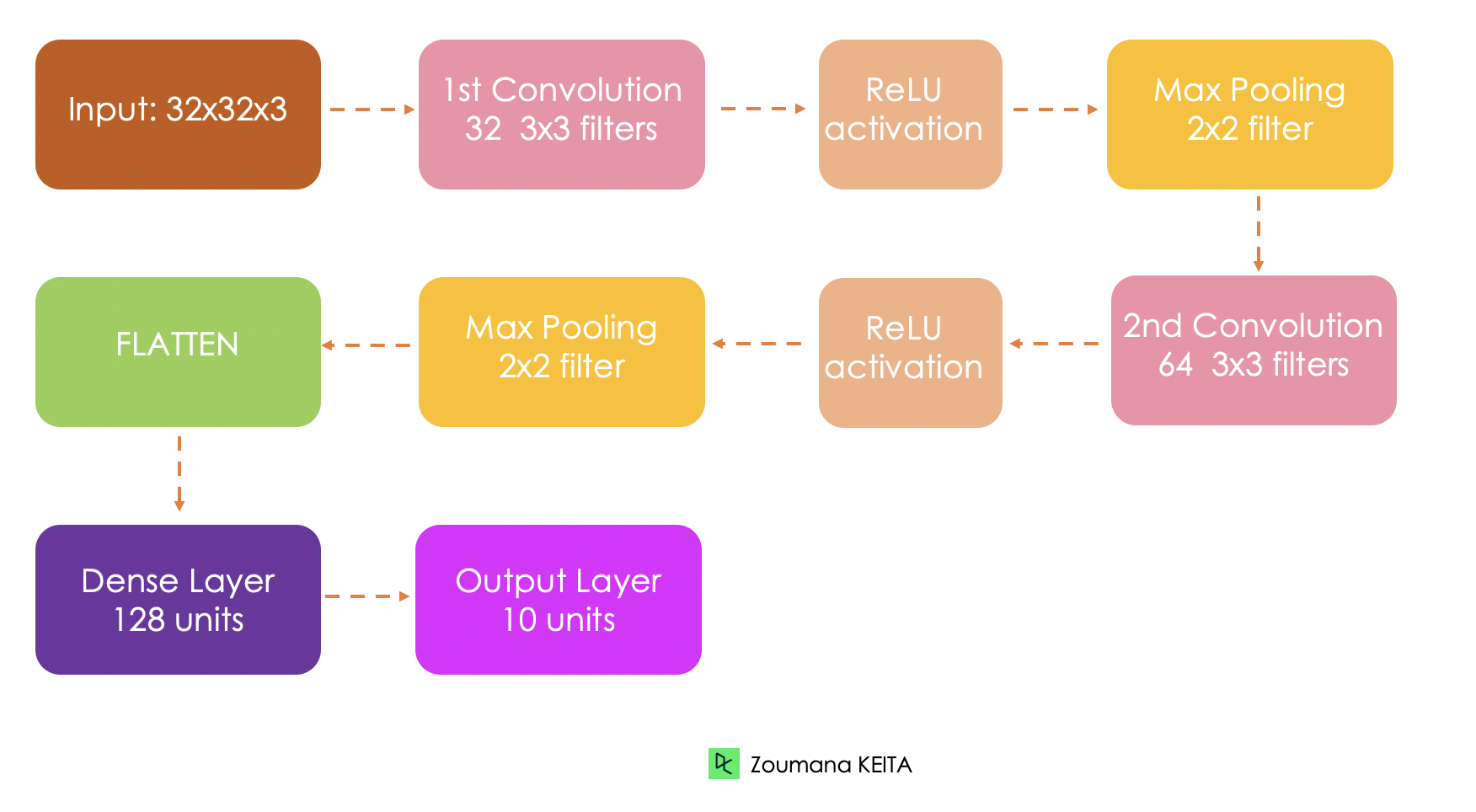
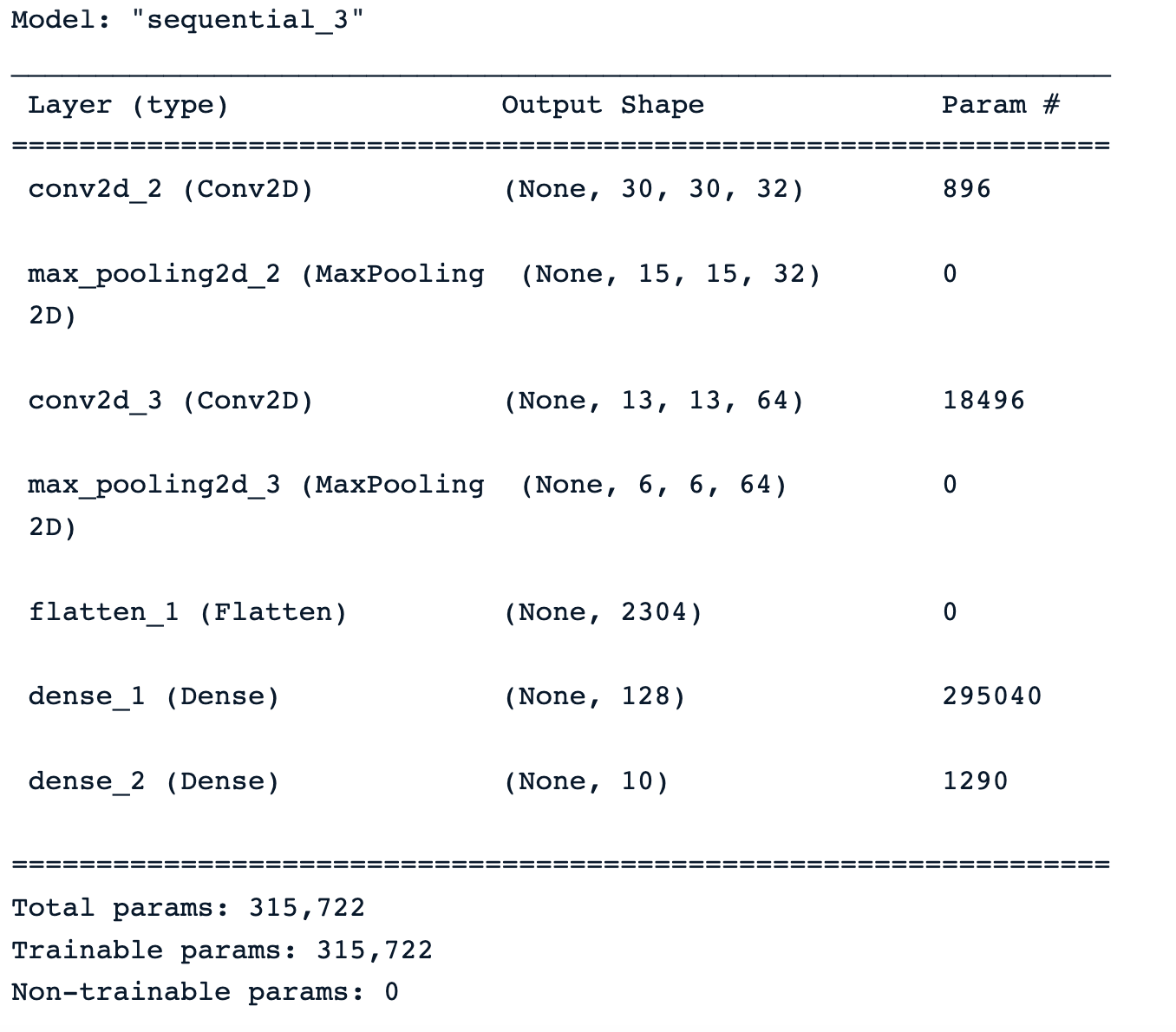
- The input of the model is a 32x32x3 tensor, respectively, for the width, height, and channels.
- We will have two convolutional layers. The first layer applies 32 filters of size 3x3 each and a ReLU activation function. And the second one applies 64 filters of size 3x3
- The first pooling layer will apply a 2x2 max pooling
- The second pooling layer will apply a 2x2 max pooling as well
- The fully connected layer will have 128 units and a ReLU activation function
- Finally, the output will be 10 units corresponding to the 10 classes, and the activation function is a softmax to generate the probability distributions.
Load dataset
The built-in dataset is loaded from the keras.datasets() as follows:
(train_images, train_labels), (test_images, test_labels) = cf10.load_data()Exploratory Data Analysis
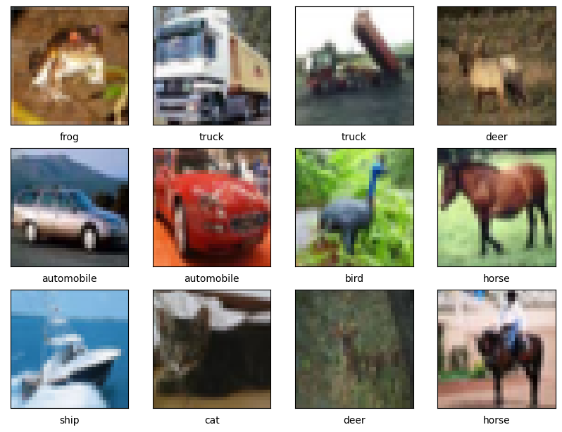
In this section, we will focus solely on showing some sample images since we already know the proportion of each class in both the training and testing data.
The helper function show_images() shows a total of 12 images by default and takes three main parameters:
- The training images
- The class names
- And the training labels.
import matplotlib.pyplot as plt

def show_images(train_images,
            	class_names,
            	train_labels,
            	nb_samples = 12, nb_row = 4):

	plt.figure(figsize=(12, 12))
	for i in range(nb_samples):
    	plt.subplot(nb_row, nb_row, i + 1)
    	plt.xticks([])
    	plt.yticks([])
    	plt.grid(False)
    	plt.imshow(train_images[i], cmap=plt.cm.binary)
    	plt.xlabel(class_names[train_labels[i][0]])
	plt.show()
Now, we can call the function with the required parameters.
class_names = ['airplane', 'automobile', 'bird', 'cat', 'deer',
           	'dog', 'frog', 'horse', 'ship', 'truck']

show_images(train_images, class_names, train_labels)
A successful execution of the previous code generates the images below.
Data preprocessing
Prior to training the model, we need to normalize the pixel values of the data in the same range (e.g. 0 to 1). This is a common preprocessing step when dealing with images to ensure scale invariance, and faster convergence during the training.
max_pixel_value = 255

train_images = train_images / max_pixel_value
test_images = test_images / max_pixel_value
Also, we notice that the labels are represented in a categorical format like cat, horse, bird, and so one. We need to convert them into a numerical format so that they can be easily processed by the neural network.
from tensorflow.keras.utils import to_categorical
train_labels = to_categorical(train_labels, len(class_names))
test_labels = to_categorical(test_labels, len(class_names))
Model architecture implementation
The next step is to implement the architecture of the network based on the previous description.
First, we define the model using the Sequential() class, and each layer is added to the model with the add() function.
from tensorflow.keras import Sequential
from tensorflow.keras.layers import Conv2D, MaxPooling2D, Flatten, Dense

# Variables
INPUT_SHAPE = (32, 32, 3)
FILTER1_SIZE = 32
FILTER2_SIZE = 64
FILTER_SHAPE = (3, 3)
POOL_SHAPE = (2, 2)
FULLY_CONNECT_NUM = 128
NUM_CLASSES = len(class_names)

# Model architecture implementation
model = Sequential()
model.add(Conv2D(FILTER1_SIZE, FILTER_SHAPE, activation='relu', input_shape=INPUT_SHAPE))
model.add(MaxPooling2D(POOL_SHAPE))
model.add(Conv2D(FILTER2_SIZE, FILTER_SHAPE, activation='relu'))
model.add(MaxPooling2D(POOL_SHAPE))
model.add(Flatten())
model.add(Dense(FULLY_CONNECT_NUM, activation='relu'))
model.add(Dense(NUM_CLASSES, activation='softmax'))
After applying the summary() function to the model, we a comprehensive summary of the model’s architecture with information about each layer, its type, output shape and the total number of trainable parameters.
Model training
All the resources are finally available to configure and trigger the training of the model. This is done respectively with the compile() and fit() functions which takes the following parameters:
- The Optimizer is responsible for updating the model’s weights and biases. In our case, we are using the Adam optimizer.
- The loss function is used to measure the misclassification errors, and we are using the Crosentropy().
- Finally, the metrics is used to measure the performance of the model, and accuracy, precision, and recall will be displayed in our use case.
from tensorflow.keras.metrics import Precision, Recall

BATCH_SIZE = 32
EPOCHS = 30

METRICS = metrics=['accuracy',
               	Precision(name='precision'),
               	Recall(name='recall')]

model.compile(optimizer='adam',
          	loss='categorical_crossentropy',
          	metrics = METRICS)

# Train the model
training_history = model.fit(train_images, train_labels,
                	epochs=EPOCHS, batch_size=BATCH_SIZE,
                	validation_data=(test_images, test_labels))
Model evaluation
After the model training, we can compare its performance on both the training and testing datasets by plotting the above metrics using the show_performance_curve() helper function in two dimensions.
- The horizontal axis (x) is the number of epochs
- The vertical one (y) is the underlying performance of the model.
- The curve represents the value of the metrics at a specific epoch.
For better visualization, a vertical red line is drawn through the intersection of the training and validation performance values along with the optimal value.
def show_performance_curve(training_result, metric, metric_label):

	train_perf = training_result.history[str(metric)]
	validation_perf = training_result.history['val_'+str(metric)]
	intersection_idx = np.argwhere(np.isclose(train_perf,
                                            	validation_perf, atol=1e-2)).flatten()[0]
	intersection_value = train_perf[intersection_idx]

	plt.plot(train_perf, label=metric_label)
	plt.plot(validation_perf, label = 'val_'+str(metric))
	plt.axvline(x=intersection_idx, color='r', linestyle='--', label='Intersection')

	plt.annotate(f'Optimal Value: {intersection_value:.4f}',
         	xy=(intersection_idx, intersection_value),
         	xycoords='data',
         	fontsize=10,
         	color='green')

	plt.xlabel('Epoch')
	plt.ylabel(metric_label)
	plt.legend(loc='lower right')
Then, the function is applied for both the accuracy and the precision of the model.
show_performance_curve(training_history, 'accuracy', 'accuracy')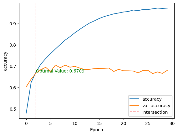
show_performance_curve(training_history, 'precision', 'precision')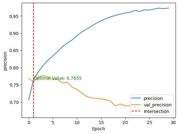
After training the model without any fine-tuning and pre-processing, we end up with:
- An accuracy score of 67.09%, meaning that the model correctly classifies 67% of the samples out of every 100 samples.
- And, a precision of 76.55%, meaning that out of each 100 positive predictions, almost 77 of them are true positives, and the remaining 23 are false positives.
- These scores are achieved respectively at the third and second epochs for accuracy and precision.
These two metrics give a global understanding of the model behavior.
What if we want to know for each class which ones are the model good at predicting and those that the model struggles with?
This can be achieved from the confusion matrix, which shows for each class the number of correct and wrong predictions. The implementation is given below. We start by making predictions on the test data, then compute the confusion matrix and show the final result.
from sklearn.metrics import confusion_matrix, ConfusionMatrixDisplay

test_predictions = model.predict(test_images)

test_predicted_labels = np.argmax(test_predictions, axis=1)

test_true_labels = np.argmax(test_labels, axis=1)

cm = confusion_matrix(test_true_labels, test_predicted_labels)

cmd = ConfusionMatrixDisplay(confusion_matrix=cm)

cmd.plot(include_values=True, cmap='viridis', ax=None, xticks_rotation='horizontal')
plt.show()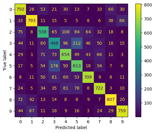
- Classes 0, 1, 6, 7, 8, 9, respectively, for airplane, automobile, frog, horse, ship, and truck have the highest values at the diagonal. This means that the model is better at predicting those classes.
- On the other hand, it seems to struggle with the remaining classes:
- The classes with the highest off-diagonal values are those the model confuses the good classes with. For instance, it confuses birds (class 2) with an airplane, and automobile with trucks (class 9).
Learn more about confusion matrix from our tutorial understanding confusion matrix in R, which takes course material from DataCamp’s Machine Learning toolbox course.
This model can be improved with additional tasks such as:
- Image augmentation
- Transfer learning using pre-trained models such as ResNet, MobileNet, or VGG. Our Transfer learning tutorial explains what transfer learning is and some of its applications in real life.
- Applying different regularization technics such as L1, L2 or dropout.
- Fine-tuning different hyperparameters such as learning rate, the batch size, number of layers in the network.
Conclusion
This article has covered a complete overview of CNNs in TensorFlow, providing details about each layer of the CNNs architecture. Also, it made a brief introduction to TensorFlow and how it helps machine learning engineers and researchers build sophisticated neural networks.
We applied all these skill sets to a real-world scenario related to a multiclass classification task.
Our beginner’s guide to object detection could be a great next step to further your learning about computer vision. It explores the key components in object detection and explains how to implement in SSD and Faster RCNN available in Tensorflow.
