What are Recurrent Neural Networks (RNN)
A recurrent neural network (RNN) is the type of artificial neural network (ANN) that is used in Apple’s Siri and Google’s voice search. RNN remembers past inputs due to an internal memory which is useful for predicting stock prices, generating text, transcriptions, and machine translation.
In the traditional neural network, the inputs and the outputs are independent of each other, whereas the output in RNN is dependent on prior elementals within the sequence. Recurrent networks also share parameters across each layer of the network. In feedforward networks, there are different weights across each node. Whereas RNN shares the same weights within each layer of the network and during gradient descent, the weights and basis are adjusted individually to reduce the loss.

The image above is a simple representation of recurrent neural networks. If we are forecasting stock prices using simple data [45,56,45,49,50,…], each input from X0 to Xt will contain a past value. For example, X0 will have 45, X1 will have 56, and these values are used to predict the next number in a sequence.
How Recurrent Neural Networks Work
In RNN, the information cycles through the loop, so the output is determined by the current input and previously received inputs.
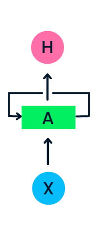
The input layer X processes the initial input and passes it to the middle layer A. The middle layer consists of multiple hidden layers, each with its activation functions, weights, and biases. These parameters are standardized across the hidden layer so that instead of creating multiple hidden layers, it will create one and loop it over.
Instead of using traditional backpropagation, recurrent neural networks use backpropagation through time (BPTT) algorithms to determine the gradient. In backpropagation, the model adjusts the parameter by calculating errors from the output to the input layer. BPTT sums the error at each time step as RNN shares parameters across each layer. Learn more on RNNs and how they work at What are Recurrent Neural Networks?.
Types of Recurrent Neural Networks
Feedforward networks have single input and output, while recurrent neural networks are flexible as the length of inputs and outputs can be changed. This flexibility allows RNNs to generate music, sentiment classification, and machine translation.
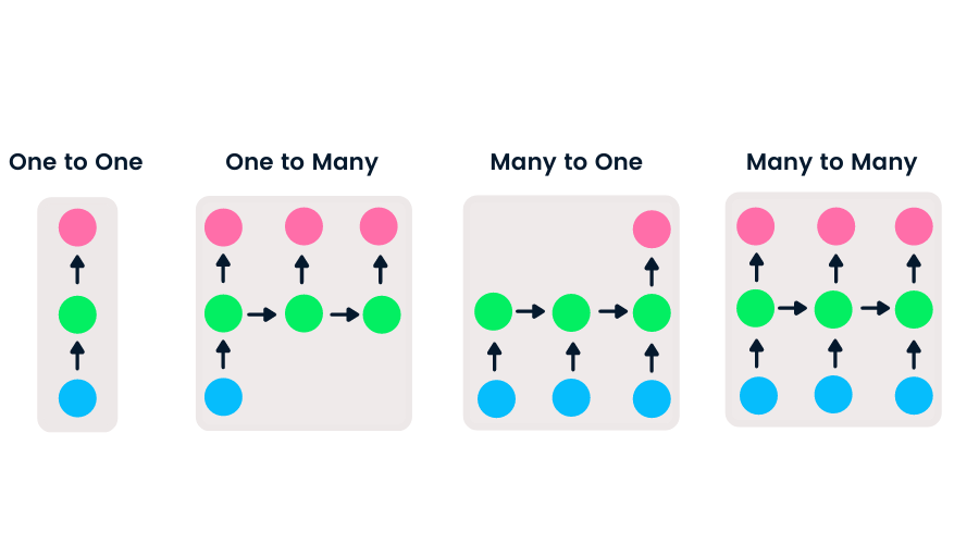
There are four types of RNN based on different lengths of inputs and outputs.
- One-to-one is a simple neural network. It is commonly used for machine learning problems that have a single input and output.
- One-to-many has a single input and multiple outputs. This is used for generating image captions.
- Many-to-one takes a sequence of multiple inputs and predicts a single output. It is popular in sentiment classification, where the input is text and the output is a category.
- Many-to-many takes multiple inputs and outputs. The most common application is machine translation.
Popular Machine Learning Courses
Introduction to Deep Learning in Python
CNN vs. RNN
The convolutional neural network (CNN) is a feed-forward neural network capable of processing spatial data. It is commonly used for computer vision applications such as image classification. The simple neural networks are good at simple binary classifications, but they can't handle images with pixel dependencies. The CNN model architecture consists of convolutional layers, ReLU layers, pooling layers, and fully connected output layers. You can learn CNN by working on a project such as Convolutional Neural Networks in Python.

Key Differences Between CNN and RNN
- CNN is applicable for sparse data like images. RNN is applicable for time series and sequential data.
- While training the model, CNN uses a simple backpropagation and RNN uses backpropagation through time to calculate the loss.
- RNN can have no restriction in length of inputs and outputs, but CNN has finite inputs and finite outputs.
- CNN has a feedforward network and RNN works on loops to handle sequential data.
- CNN can also be used for video and image processing. RNN is primarily used for speech and text analysis.
Limitations of RNN
Simple RNN models usually run into two major issues. These issues are related to gradient, which is the slope of the loss function along with the error function.
- Vanishing Gradient problem occurs when the gradient becomes so small that updating parameters becomes insignificant; eventually the algorithm stops learning.
- Exploding Gradient problem occurs when the gradient becomes too large, which makes the model unstable. In this case, larger error gradients accumulate, and the model weights become too large. This issue can cause longer training times and poor model performance.
The simple solution to these issues is to reduce the number of hidden layers within the neural network, which will reduce some complexity in RNNs. These issues can also be solved by using advanced RNN architectures such as LSTM and GRU.
RNN Advanced Architectures
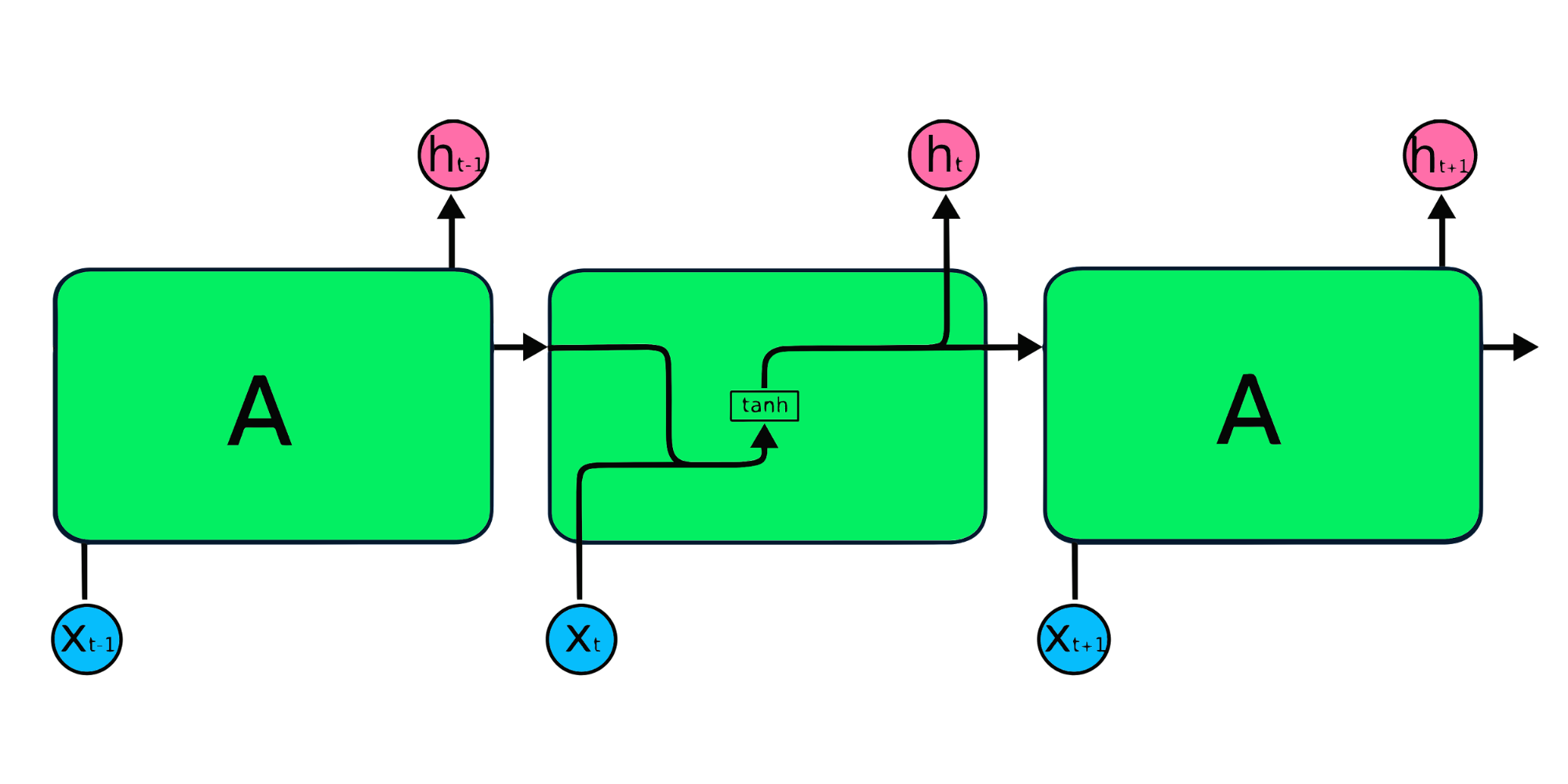
The simple RNN repeating modules have a basic structure with a single tanh layer. RNN simple structure suffers from short memory, where it struggles to retain previous time step information in larger sequential data. These problems can easily be solved by long short term memory (LSTM) and gated recurrent unit (GRU), as they are capable of remembering long periods of information.
Long Short Term Memory (LSTM)
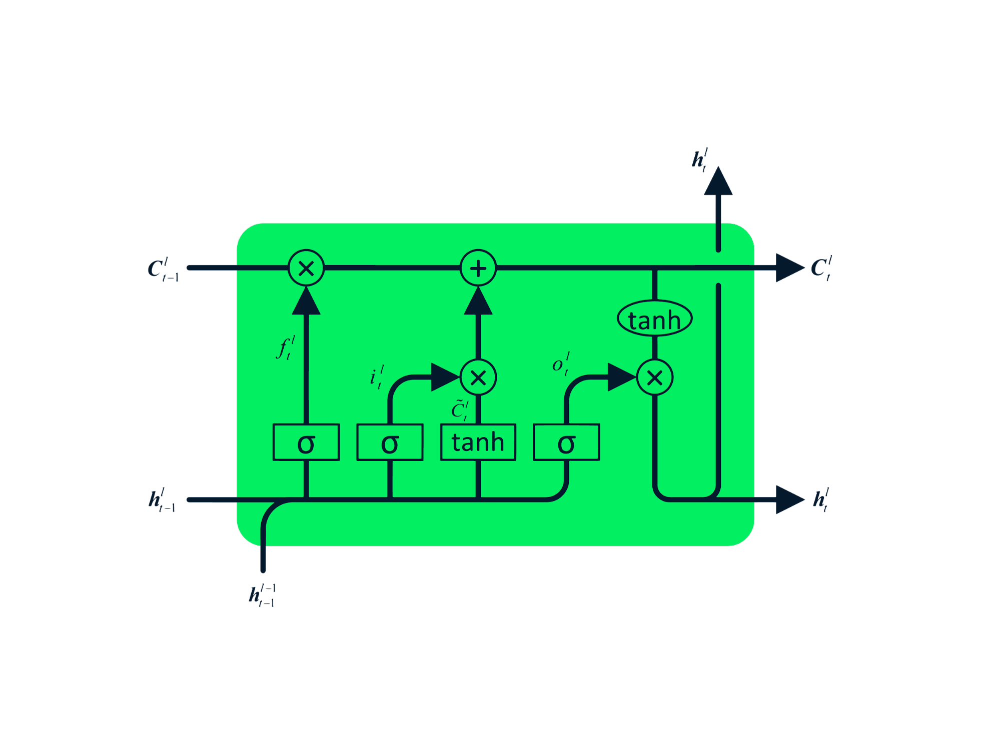
The Long Short Term Memory (LSTM) is the advanced type of RNN, which was designed to prevent both decaying and exploding gradient problems. Just like RNN, LSTM has repeating modules, but the structure is different. Instead of having a single layer of tanh, LSTM has four interacting layers that communicate with each other. This four-layered structure helps LSTM retain long-term memory and can be used in several sequential problems including machine translation, speech synthesis, speech recognition, and handwriting recognition. You can gain hands-on experience in LSTM by following the guide: Python LSTM for Stock Predictions.
Gated Recurrent Unit (GRU)
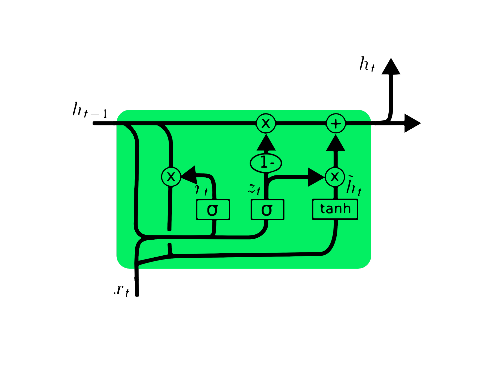
The gated recurrent unit (GRU) is a variation of LSTM as both have design similarities, and in some cases, they produce similar results. GRU uses an update gate and reset gate to solve the vanishing gradient problem. These gates decide what information is important and pass it to the output. The gates can be trained to store information from long ago, without vanishing over time or removing irrelevant information.
Unlike LSTM, GRU does not have cell state Ct. It only has a hidden state ht, and due to the simple architecture, GRU has a lower training time compared to LSTM models. The GRU architecture is easy to understand as it takes input xt and the hidden state from the previous timestamp ht-1 and outputs the new hidden state ht. You can get in-depth knowledge about GRU at Understanding GRU Networks.
MasterCard Stock Price Prediction Using LSTM & GRU
In this project, we are going to use Kaggle’s MasterCard stock dataset from May-25-2006 to Oct-11-2021 and train the LSTM and GRU models to forecast the stock price. This is a simple project-based tutorial where we will analyze data, preprocess the data to train it on advanced RNN models, and finally evaluate the results.
The project requires Pandas and Numpy for data manipulation, Matplotlib.pyplot for data visualization, scikit-learn for scaling and evaluation, and TensorFlow for modeling. We will also set seeds for reproducibility.
# Importing the libraries
import numpy as np
import pandas as pd
import matplotlib.pyplot as plt

from sklearn.preprocessing import MinMaxScaler
from sklearn.metrics import mean_squared_error

from tensorflow.keras.models import Sequential
from tensorflow.keras.layers import Dense, LSTM, Dropout, GRU, Bidirectional
from tensorflow.keras.optimizers import SGD
from tensorflow.random import set_seed

set_seed(455)
np.random.seed(455)
Data Analysis
In this part, we will import the MasterCard dataset by adding the Date column to the index and converting it to DateTime format. We will also drop irrelevant columns from the dataset as we are only interested in stock prices, volume, and date.
The dataset has Date as index and Open, High, Low, Close, and Volume as columns. It looks like we have successfully imported a cleaned dataset.
dataset = pd.read_csv(
    "data/Mastercard_stock_history.csv", index_col="Date", parse_dates=["Date"]
).drop(["Dividends", "Stock Splits"], axis=1)
print(dataset.head())
               Open      High       Low     Close     Volume
Date
2006-05-25  3.748967  4.283869  3.739664  4.279217  395343000
2006-05-26  4.307126  4.348058  4.103398  4.179680  103044000
2006-05-30  4.183400  4.184330  3.986184  4.093164   49898000
2006-05-31  4.125723  4.219679  4.125723  4.180608   30002000
2006-06-01  4.179678  4.474572  4.176887  4.419686   62344000
The .describe() function helps us analyze the data in depth. Let’s focus on the High column as we are going to use it to train the model. We can also choose Close or Open columns for a model feature, but High makes more sense as it provides us information of how high the values of the share went on the given day.
The minimum stock price is $4.10, and the highest is $400.5. The mean is at $105.9 and the standard deviation $107.3, which means that stocks have high variance.
print(dataset.describe())
             Open         High          Low        Close        Volume
count  3872.000000  3872.000000  3872.000000  3872.000000  3.872000e+03
mean    104.896814   105.956054   103.769349   104.882714  1.232250e+07
std     106.245511   107.303589   105.050064   106.168693  1.759665e+07
min       3.748967     4.102467     3.739664     4.083861  6.411000e+05
25%      22.347203    22.637997    22.034458    22.300391  3.529475e+06
50%      70.810079    71.375896    70.224002    70.856083  5.891750e+06
75%     147.688448   148.645373   146.822013   147.688438  1.319775e+07
max     392.653890   400.521479   389.747812   394.685730  3.953430e+08
By using .isna().sum() we can determine the missing values in the dataset. It seems that the dataset has no missing values.
dataset.isna().sum()
Open      0
High      0
Low       0
Close     0
Volume    0
dtype: int64
The train_test_plot function takes three arguments: dataset, tstart, and tend and plots a simple line graph. The tstart and tend are time limits in years. We can change these arguments to analyze specific periods. The line plot is divided into two parts: train and test. This will allow us to decide the distribution of the test dataset.
MasterCard stock prices have been on the rise since 2016. It had a dip in the first quarter of 2020 but it gained a stable position in the latter half of the year. Our test dataset consists of one year, from 2021 to 2022, and the rest of the dataset is used for training.
tstart = 2016
tend = 2020

def train_test_plot(dataset, tstart, tend):
    dataset.loc[f"{tstart}":f"{tend}", "High"].plot(figsize=(16, 4), legend=True)
    dataset.loc[f"{tend+1}":, "High"].plot(figsize=(16, 4), legend=True)
    plt.legend([f"Train (Before {tend+1})", f"Test ({tend+1} and beyond)"])
    plt.title("MasterCard stock price")
    plt.show()

train_test_plot(dataset,tstart,tend)

Data Preprocessing
The train_test_split function divides the dataset into two subsets: training_set and test_set.
def train_test_split(dataset, tstart, tend):
    train = dataset.loc[f"{tstart}":f"{tend}", "High"].values
    test = dataset.loc[f"{tend+1}":, "High"].values
    return train, test
training_set, test_set = train_test_split(dataset, tstart, tend)
We will use the MinMaxScaler function to standardize our training set, which will help us avoid the outliers or anomalies. You can also try using StandardScaler or any other scalar function to normalize your data and improve model performance.
sc = MinMaxScaler(feature_range=(0, 1))
training_set = training_set.reshape(-1, 1)
training_set_scaled = sc.fit_transform(training_set)
The split_sequence function uses a training dataset and converts it into inputs (X_train) and outputs (y_train).
For example, if the sequence is [1,2,3,4,5,6,7,8,9,10,11,12] and the n_step is three, then it will convert the sequence into three input timestamps and one output as shown below:
| X | y |
|---|---|
| 1,2,3 | 4 |
| 2,3,4 | 5 |
| 3,4,5 | 6 |
| 4,5,6 | 7 |
| … | … |
In this project, we are using 60 n_steps. We can also reduce or increase the number of steps to optimize model performance.
def split_sequence(sequence, n_steps):
    X, y = list(), list()
    for i in range(len(sequence)):
        end_ix = i + n_steps
        if end_ix > len(sequence) - 1:
            break
        seq_x, seq_y = sequence[i:end_ix], sequence[end_ix]
        X.append(seq_x)
        y.append(seq_y)
    return np.array(X), np.array(y)


n_steps = 60
features = 1
# split into samples
X_train, y_train = split_sequence(training_set_scaled, n_steps)
We are working with univariate series, so the number of features is one, and we need to reshape the X_train to fit on the LSTM model. The X_train has [samples, timesteps], and we will reshape it to [samples, timesteps, features].
# Reshaping X_train for model
X_train = X_train.reshape(X_train.shape[0],X_train.shape[1],features)
LSTM Model
The model consists of a single hidden layer of LSTM and an output layer. You can experiment with the number of units, as more units will give you better results. For this experiment, we will set LSTM units to 125, tanh as activation, and set input size.
Author’s Note: Tensorflow library is user-friendly, so we don't have to create LSTM or GRU models from scratch. We will simply use the LSTM or GRU modules to construct the model.
Finally, we will compile the model with an RMSprop optimizer and mean square error as a loss function.
# The LSTM architecture
model_lstm = Sequential()
model_lstm.add(LSTM(units=125, activation="tanh", input_shape=(n_steps, features)))
model_lstm.add(Dense(units=1))
# Compiling the model
model_lstm.compile(optimizer="RMSprop", loss="mse")

model_lstm.summary()
Model: "sequential"
_________________________________________________________________
Layer (type)                 Output Shape              Param #
=================================================================
lstm (LSTM)                  (None, 125)               63500
_________________________________________________________________
dense (Dense)                (None, 1)                 126
=================================================================
Total params: 63,626
Trainable params: 63,626
Non-trainable params: 0
_________________________________________________________________
The model will train on 50 epochs with 32 batch sizes. You can change the hyperparameters to reduce training time or improve the results. The model training was successfully completed with the best possible loss.
model_lstm.fit(X_train, y_train, epochs=50, batch_size=32)
Epoch 50/50
38/38 [==============================] - 1s 30ms/step - loss: 3.1642e-04
Results
We are going to repeat preprocessing and normalize the test set. First of all we will transform then split the dataset into samples, reshape it, predict, and inverse transform the predictions into standard form.
dataset_total = dataset.loc[:,"High"]
inputs = dataset_total[len(dataset_total) - len(test_set) - n_steps :].values
inputs = inputs.reshape(-1, 1)
#scaling
inputs = sc.transform(inputs)

# Split into samples
X_test, y_test = split_sequence(inputs, n_steps)
# reshape
X_test = X_test.reshape(X_test.shape[0], X_test.shape[1], features)
#prediction
predicted_stock_price = model_lstm.predict(X_test)
#inverse transform the values
predicted_stock_price = sc.inverse_transform(predicted_stock_price)
The plot_predictions function will plot a real versus predicted line chart. This will help us visualize the difference between actual and predicted values.
The return_rmse function takes in test and predicted arguments and prints out the root mean square error (rmse) metric.
def plot_predictions(test, predicted):
    plt.plot(test, color="gray", label="Real")
    plt.plot(predicted, color="red", label="Predicted")
    plt.title("MasterCard Stock Price Prediction")
    plt.xlabel("Time")
    plt.ylabel("MasterCard Stock Price")
    plt.legend()
    plt.show()


def return_rmse(test, predicted):
    rmse = np.sqrt(mean_squared_error(test, predicted))
    print("The root mean squared error is {:.2f}.".format(rmse))
According to the line plot below, the single-layered LSTM model has performed well.
plot_predictions(test_set,predicted_stock_price)
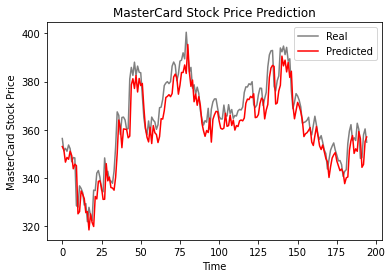
The results look promising as the model got 6.70 rmse on the test dataset.
return_rmse(test_set,predicted_stock_price)
>>> The root mean squared error is 6.70.
GRU Model
We are going to keep everything the same and just replace the LSTM layer with the GRU layer to properly compare the results. The model structure contains a single GRU layer with 125 units and an output layer.
model_gru = Sequential()
model_gru.add(GRU(units=125, activation="tanh", input_shape=(n_steps, features)))
model_gru.add(Dense(units=1))
# Compiling the RNN
model_gru.compile(optimizer="RMSprop", loss="mse")

model_gru.summary()
Model: "sequential_5"
_________________________________________________________________
Layer (type)                 Output Shape              Param #
=================================================================
gru_4 (GRU)                  (None, 125)               48000
_________________________________________________________________
dense_5 (Dense)              (None, 1)                 126
=================================================================
Total params: 48,126
Trainable params: 48,126
Non-trainable params: 0
_________________________________________________________________
The model has successfully trained with 50 epochs and a batch size of 32.
model_gru.fit(X_train, y_train, epochs=50, batch_size=32)
Epoch 50/50
38/38 [==============================] - 1s 29ms/step - loss: 2.6691e-04
Results
As we can see, the real and predicted values are relatively close. The predicted line chart almost fits the actual values.
GRU_predicted_stock_price = model_gru.predict(X_test)
GRU_predicted_stock_price = sc.inverse_transform(GRU_predicted_stock_price)
plot_predictions(test_set, GRU_predicted_stock_price)
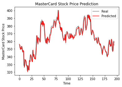
GRU model got 5.50 rmse on the test dataset, which is an improvement from the LSTM model.
return_rmse(test_set,GRU_predicted_stock_price)
>>> The root mean squared error is 5.50.
Conclusion
The world is moving towards hybrid solutions where data scientists are using CNN-RNN hybrid networks in the field of image captioning, emotion detection, video subtitling, and DNA sequencing. Hybrid networks provide both visual and temporal characteristics for the model. Learn more about RNN by taking the course: Recurrent Neural Networks for Language Modeling in Python.
The first half of the tutorial covers the basics of recurrent neural networks, its limitations, and solutions in the form of more advanced architecture. The second half of the tutorial is about developing MasterCard stock price predictions using LSTM and GRU models. The results clearly show that the GRU model performed better than LSTM, with a similar structure and hyperparameters.
This project is available on the DataCamp workspace.
