Arsitektur ResNet: Residual Network dan Skip Connection

Jaringan saraf yang lebih dalam seharusnya berkinerja lebih baik. Namun dalam praktiknya, itu tidak selalu terjadi.

Setelah kedalaman tertentu, akurasi justru bisa menurun. Bukan karena model overfitting - melainkan karena proses pelatihannya sendiri yang gagal. Gradien cenderung menghilang sebelum mencapai lapisan awal, dan lapisan-lapisan tersebut berhenti belajar. Anda mungkin mengira menambah lebih banyak lapisan akan memperbaikinya, tetapi sering kali justru memperburuk keadaan.

ResNet memperbaikinya dengan gagasan inti berupa skip connection. Alih-alih memaksa setiap lapisan untuk belajar dari nol, ia memungkinkan jaringan melompati lapisan dan menambahkan input langsung ke output.

Dalam artikel ini, saya akan membahas cara kerja ResNet, seperti apa arsitekturnya, dan mengapa ini masih menjadi algoritme andalan dalam deep learning modern.

Ingin melihat ResNet dalam praktik? Selesaikan latihan klasifikasi gambar dengan ResNet sebagai bagian dari kursus Deep Learning for Images with PyTorch.

Apa Itu Arsitektur ResNet?

ResNet - singkatan dari Residual Network - adalah arsitektur jaringan saraf yang dirancang untuk membuat pelatihan jaringan yang dalam menjadi praktis.

Gagasan ini diperkenalkan oleh Microsoft Research pada tahun 2015. Algoritme ini menggunakan residual connection untuk mengatasi masalah pelatihan yang membatasi jaringan dalam saat itu. Idunya sederhana, tetapi setelah penemuan tersebut, untuk pertama kalinya Anda dapat melatih jaringan dengan 50, 101, bahkan 152 lapisan secara andal - tanpa melihat kinerja menurun.

Sebelum ResNet, mencapai kedalaman sedalam itu sebenarnya bukan pilihan.

Mengapa Jaringan Dalam Sulit Dilatih

Lebih banyak lapisan seharusnya memberi lebih banyak peluang bagi jaringan untuk belajar. Dalam praktiknya, setelah kedalaman tertentu, semuanya mulai kacau.

Ada dua masalah yang berperan di sini.

Yang pertama adalah masalah gradien menghilang (vanishing gradient). Jaringan saraf belajar dengan mengirimkan sinyal galat ke belakang melalui jaringan - proses ini disebut backpropagation. Setiap lapisan menyesuaikan bobotnya berdasarkan sinyal tersebut. Namun saat sinyal itu berjalan mundur melalui banyak lapisan, sinyal dikalikan oleh bilangan kecil berulang kali, lalu menyusut. Ketika mencapai lapisan awal, hampir tidak ada yang tersisa. Lapisan-lapisan itu berhenti memperbarui, artinya berhenti belajar.

Yang kedua adalah masalah degradasi. Ini berlawanan dengan intuisi. Anda akan berharap jaringan 56 lapisan setidaknya berkinerja sama baiknya dengan yang 20 lapisan - toh kapasitasnya lebih besar. Namun para peneliti menemukan hal sebaliknya. Jaringan yang lebih dalam berkinerja lebih buruk, bahkan pada data pelatihan. Itu menyingkirkan overfitting sebagai penyebabnya. Model bukan terlalu banyak menghafal. Sebaliknya, model kesulitan melakukan optimisasi.

Inilah pembedanya yang penting. Ini bukan masalah generalisasi yang dapat Anda perbaiki dengan dropout atau regularisasi. Ini masalah optimisasi - jaringan tidak dapat menemukan bobot yang baik sejak awal.

ResNet dirancang untuk menyelesaikan dua masalah ini. Mari saya tunjukkan caranya.

Gagasan Inti: Pembelajaran Residual

Jaringan saraf tradisional mencoba mempelajari pemetaan langsung dari input ke output. Setiap lapisan melihat apa yang masuk lalu mencoba menebak apa yang harus keluar. Itu bekerja baik untuk jaringan yang dangkal. Namun saat Anda membuatnya lebih dalam, Anda bertemu dua masalah yang dibahas sebelumnya.

Dengan ResNet, alih-alih meminta setiap blok mempelajari pemetaan penuh, ia mengajukan pertanyaan yang lebih sederhana: apa yang perlu saya tambahkan ke input untuk mendapatkan output yang benar?

Perbedaan itu disebut residual.

Jadi alih-alih mempelajari:

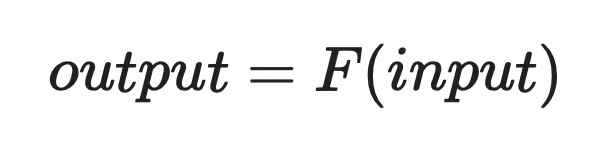
Residual learning (1)

Jaringan mempelajari:

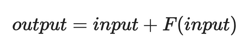
Residual learning (2)

Di mana F(input) adalah residual - koreksi kecil yang perlu dibuat jaringan. Jika lapisan tidak perlu mengubah apa pun, ia bisa mendorong F(input) menuju nol dan meneruskan input apa adanya.

Ini mungkin terdengar seperti penyetelan kecil. Namun ini mengubah apa yang harus dipelajari jaringan. Mempelajari koreksi kecil adalah masalah optimisasi yang jauh lebih mudah daripada mempelajari transformasi penuh dari nol, dan itulah yang membuat jaringan yang lebih dalam dapat dilatih.

Apa Itu Skip Connection di ResNet?

Skip connection adalah persis seperti namanya - jalur langsung yang melewati satu atau lebih lapisan dan memberi makan input ke titik yang lebih jauh di jaringan.

Dalam jaringan tradisional, data mengalir melalui setiap lapisan secara berurutan. Setiap lapisan mentransformasikan input dan meneruskan hasilnya ke lapisan berikutnya. Skip connection mengambil input asli dan menambahkannya langsung ke output dari lapisan yang lebih jauh dalam blok.

Berikut cara sederhana untuk membayangkannya:

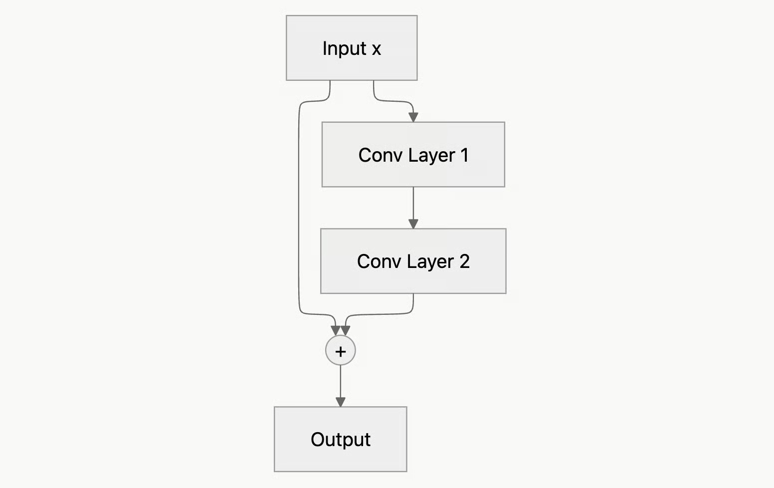
Contoh grafik skip connection

Input x menempuh dua jalur sekaligus. Satu jalur melalui lapisan konvolusional, yang mempelajari residual F(x). Jalur lainnya melewati lapisan tersebut dan terhubung ke tahap penjumlahan. Output akhir adalah F(x) + x.

Shortcut ini melakukan hal penting untuk pelatihan. Selama backpropagation, gradien dapat berjalan mundur melalui skip connection tanpa melewati lapisan perantara. Itu memberi lapisan awal sinyal yang lebih bersih dan kuat untuk dipelajari - persis yang kurang pada jaringan dalam sebelum ResNet.

Struktur Blok ResNet

Blok residual adalah unit berulang yang membentuk ResNet. Jika Anda memahami satu blok, Anda memahami seluruh jaringan.

Berikut yang terjadi di dalam satu blok:

1. Input x masuk ke blok dan terbagi menjadi dua jalur

2. Satu jalur melalui dua lapisan konvolusional, masing-masing diikuti oleh batch normalization dan aktivasi ReLU

3. Jalur lainnya melewati lapisan-lapisan tersebut - inilah skip connection

4. Kedua jalur bertemu pada tahap penjumlahan, di mana input asli ditambahkan ke output dari lapisan konvolusional

5. Aktivasi ReLU terakhir diterapkan pada hasilnya

Atau dalam bentuk diagram:

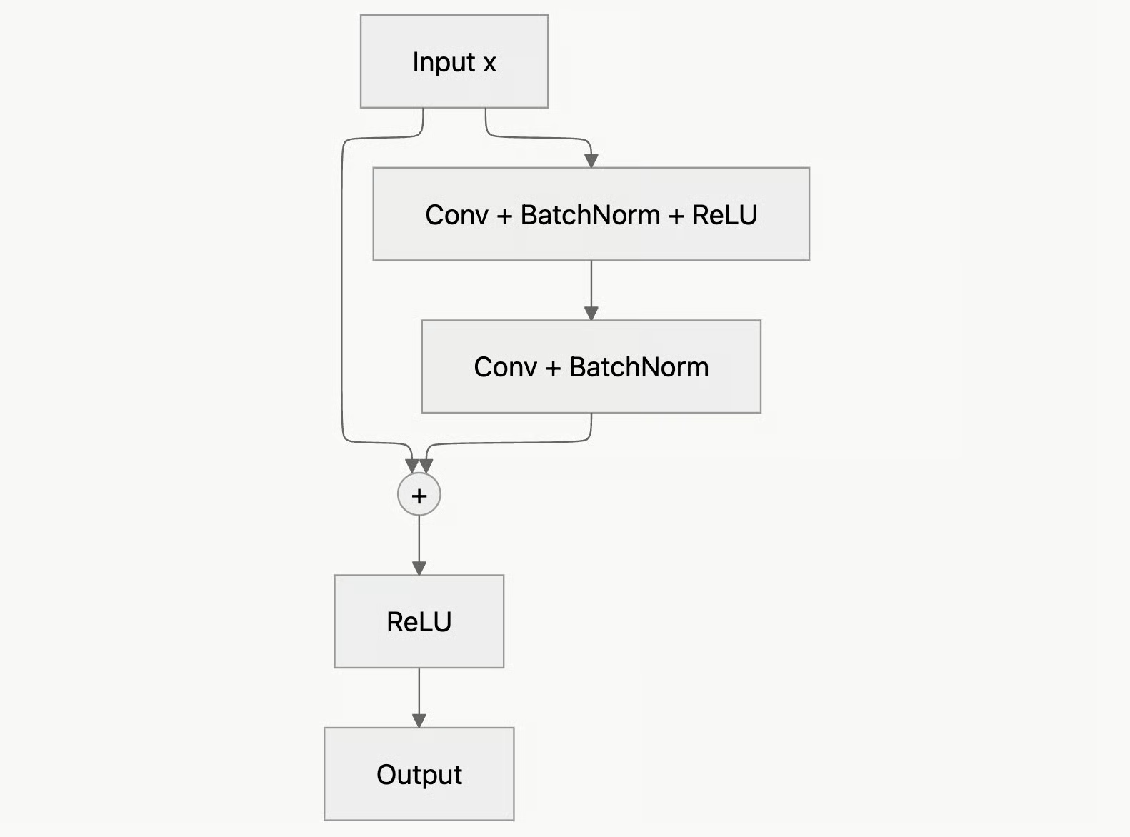
Diagram blok ResNet

Skip connection di sini disebut pemetaaan identitas (identity mapping) - input diteruskan tanpa perubahan dan ditambahkan langsung ke output yang dipelajari. Ini adalah shortcut sesederhana mungkin tanpa transformasi dan tanpa parameter tambahan.

Namun agar penjumlahan berfungsi, kedua jalur harus menghasilkan tensor dengan bentuk yang sama. Jika lapisan konvolusional mengubah dimensi spasial atau jumlah kanal, input x tidak bisa dijumlahkan. Dalam kasus tersebut, ResNet menerapkan projection shortcut - konvolusi 1×1 pada jalur skip yang membentuk ulang x agar cocok.

Kebanyakan blok dalam ResNet menggunakan identity shortcut. Projection shortcut hanya muncul ketika dimensi berubah, biasanya saat jaringan berpindah antar tahap.

Jenis-Jenis Arsitektur ResNet

ResNet hadir dalam beberapa varian standar, masing-masing dinamai berdasarkan jumlah total lapisannya. Pilihan yang tepat bergantung pada apa yang Anda optimalkan - kecepatan, akurasi, atau di antara keduanya.

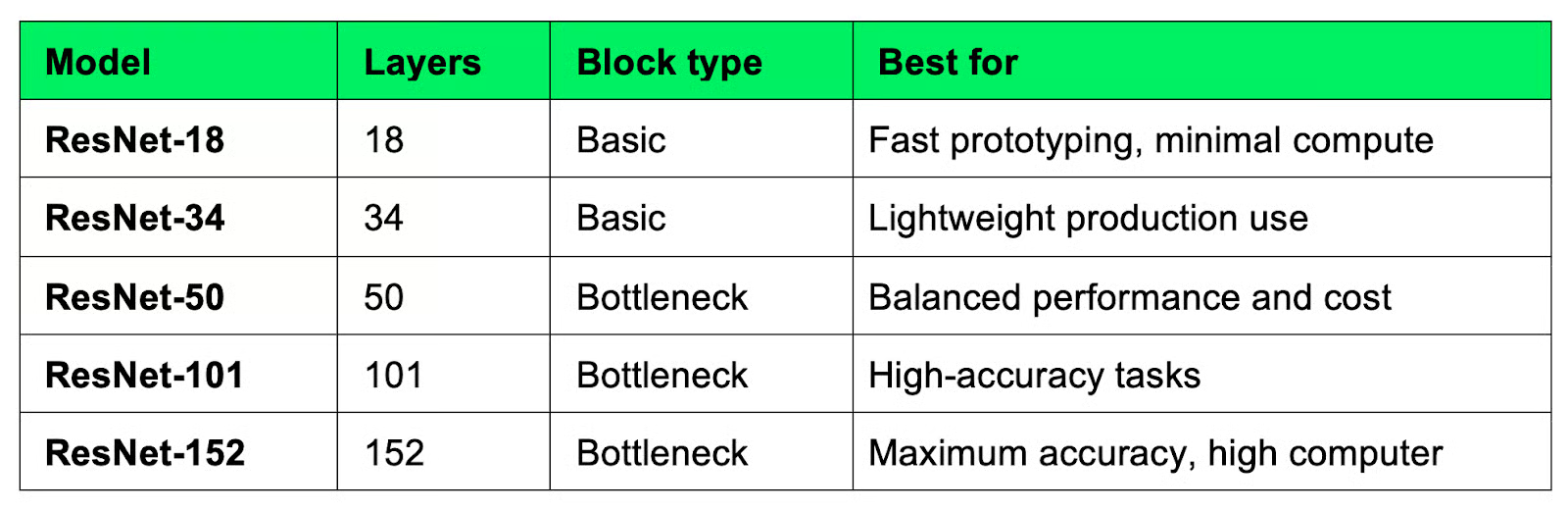
Perbandingan arsitektur ResNet

ResNet-18 dan ResNet-34 menggunakan basic block standar - dua lapisan konvolusi 3×3 dengan skip connection. Keduanya cepat dan murah dijalankan, sehingga cocok sebagai titik awal saat Anda membuat prototipe atau bekerja dengan perangkat keras terbatas.

ResNet-50 ke atas beralih ke desain berbeda yang disebut bottleneck block, yang menggunakan tiga lapisan alih-alih dua. Perubahan itu membuat jaringan yang lebih dalam lebih mudah dilatih tanpa lonjakan biaya komputasi yang sebanding. Anda akan membaca lebih lanjut cara kerjanya di bagian berikutnya.

ResNet-101 dan ResNet-152 melangkah lebih jauh dengan biaya waktu pelatihan yang lebih lama dan penggunaan memori lebih tinggi. Keduanya umum digunakan dalam riset dan sistem produksi di mana akurasi lebih penting daripada kecepatan.

Untuk sebagian besar pekerjaan praktis, ResNet-50 adalah titik awal default. Ia memiliki keseimbangan yang baik antara kedalaman dan biaya, serta didukung dengan baik di semua kerangka kerja deep learning utama.

Arsitektur Bottleneck ResNet

ResNet yang lebih dalam tidak menggunakan desain blok yang sama dengan yang lebih dangkal. Mulai dari ResNet-50, arsitektur beralih ke bottleneck block, yaitu desain tiga lapisan yang menjaga komputasi tetap terkendali seiring bertambahnya kedalaman.

Blok ini menggunakan tiga konvolusi berturut-turut:

• Konvolusi 1×1 - mengurangi jumlah kanal, membuat input lebih kecil
• Konvolusi 3×3 - melakukan pembelajaran fitur pada representasi yang lebih kecil tersebut
• Konvolusi 1×1 - memperluas kembali kanal ke ukuran semula

Konvolusi 1×1 pertama dan terakhir bertindak sebagai bottleneck - karenanya namanya. Keduanya mengompresi data sebelum konvolusi 3×3 yang lebih mahal dijalankan, lalu mengembalikannya setelahnya.

Konvolusi 3×3 pada input dengan kanal tinggi secara komputasional berat. Dengan mengurangi kanal terlebih dahulu, bottleneck block memungkinkan lapisan 3×3 bekerja pada input yang jauh lebih kecil. Hasilnya adalah blok yang dapat dibuat lebih dalam tanpa lonjakan biaya komputasi yang sebanding.

Skip connection bekerja sama seperti pada basic block - input ditambahkan ke output sebelum aktivasi terakhir. Satu-satunya perbedaannya adalah projection shortcut hampir selalu diperlukan di sini, karena dimensi kanal berubah di dalam blok.

Bagaimana ResNet Mengatasi Masalah Gradien Menghilang

Masalah gradien menghilang bermuara pada jarak. Semakin jauh gradien harus menempuh jaringan, semakin ia menyusut - dan ketika mencapai lapisan awal, tidak banyak sinyal yang tersisa untuk dipelajari.

Skip connection mengatasi masalah ini dengan memberi gradien jalur yang lebih pendek untuk dilalui.

Selama backpropagation, gradien tidak harus melewati setiap lapisan secara berurutan. Gradien dapat berjalan mundur melalui skip connection secara langsung, sepenuhnya melewati lapisan konvolusional. Shortcut tersebut menjaga gradien tetap cukup besar untuk benar-benar memperbarui lapisan awal.

Ini juga mengubah apa yang harus dipelajari setiap blok. Alih-alih menemukan transformasi penuh dari nol, jaringan hanya perlu mempelajari koreksi kecil di atas input. Itu masalah optimisasi yang jauh lebih mudah, dan artinya jaringan bisa menjadi lebih dalam tanpa pelatihan menjadi tidak stabil.

Singkatnya, jaringan yang sebelumnya terlalu dalam untuk dilatih secara andal menjadi dapat dilatih.

ResNet vs Arsitektur CNN Tradisional

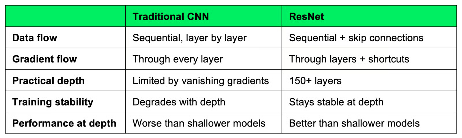
CNN tradisional dan ResNet sama-sama mempelajari fitur dari gambar, tetapi caranya berbeda.

Dalam CNN tradisional, data mengalir melalui lapisan secara garis lurus. Setiap lapisan mengambil output dari lapisan sebelumnya, menerapkan transformasi, dan meneruskan hasilnya. Itu bekerja baik sampai titik tertentu. Setelah melewati kedalaman tertentu, struktur berurutan menjadi tidak andal saat backpropagation - gradien menyusut, lapisan awal berhenti belajar, dan akurasi mulai menurun.

ResNet tidak berjalan lurus. Skip connection memungkinkan input melewati satu atau lebih lapisan dan ditambahkan langsung ke output lebih jauh di dalam blok. Jaringan masih mempelajari transformasi, tetapi juga memiliki jalur langsung bagi data dan gradien untuk mengalir.

Berikut perbandingan kedua pendekatan tersebut:

ResNet versus CNN tradisional

Skip connection membantu dengan gradien dan membuat optimisasi lebih mulus, yang berarti jaringan menemukan bobot yang baik lebih cepat dan lebih andal.

Aplikasi Arsitektur ResNet

Arsitektur ResNet digunakan di berbagai tugas dunia nyata.

Klasifikasi gambar adalah tempat ResNet bermula. Ia memenangkan ImageNet Large Scale Visual Recognition Challenge pada tahun 2015, dan masih menjadi pilihan utama untuk mengklasifikasikan gambar ke dalam kategori, baik itu citra medis, citra satelit, atau foto produk.

Deteksi objek sering menggunakan ResNet. Kerangka seperti Faster R-CNN dan Mask R-CNN menggabungkan ResNet dengan detection head yang mengidentifikasi dan melokalisasi objek dalam gambar. ResNet melakukan ekstraksi fitur dan detection head mengerjakan sisanya.

Transfer learning adalah tempat ResNet benar-benar bermanfaat bagi kebanyakan data scientist. Alih-alih melatih dari nol - yang memakan waktu berhari-hari dan banyak data - Anda memuat ResNet yang sudah dilatih sebelumnya di ImageNet dan menyetelnya kembali pada dataset Anda sendiri. Bobot pralatih sudah memuat fitur tingkat rendah yang berguna seperti tepi, tekstur, dan bentuk, sehingga Anda memulai dari posisi yang jauh lebih baik.

Ekstraksi fitur mengambil pendekatan serupa. Anda menjalankan gambar melalui ResNet pralatih dan mengambil output dari salah satu lapisan akhir. Output tersebut adalah representasi padat dan bermakna dari gambar Anda yang dapat diberi input ke pengklasifikasi atau algoritme klaster yang lebih sederhana.

Dalam semua kasus penggunaan ini, ResNet bekerja sebagai titik awal pralatih. Sebagian besar kerangka kerja deep learning hadir dengan bobot ResNet pralatih siap pakai, sehingga ini menjadi salah satu arsitektur termudah untuk mulai digunakan.

Kelebihan dan Keterbatasan ResNet

ResNet merupakan langkah maju nyata dalam deep learning - tetapi seperti arsitektur lainnya, ia memiliki trade-off. Izinkan saya membahas beberapa kelebihan dan kekurangannya.

Kelebihan

Yang paling jelas adalah kedalaman. Skip connection memungkinkan data scientist melatih jaringan dengan 50, 100, atau bahkan 150+ lapisan tanpa menghadapi masalah degradasi. Itu sebelumnya tidak dapat dilakukan secara andal sebelum ResNet.

Pelatihan juga lebih stabil. Jalur shortcut memberi gradien rute yang bersih kembali melalui jaringan, yang berarti lebih sedikit penyetelan, lebih jarang kolaps, dan hasil yang lebih dapat diprediksi di berbagai tugas dan dataset.

Dan kinerja juga menjadi keunggulan. Varian ResNet secara konsisten berada di peringkat baik pada tolok ukur gambar, dan model ResNet pralatih mudah ditransfer ke domain baru, itulah mengapa masih menjadi titik awal default untuk begitu banyak proyek visi komputer.

Keterbatasan

ResNet berat secara komputasional. Varian yang lebih dalam seperti ResNet-101 dan ResNet-152 membutuhkan banyak memori dan daya pemrosesan, yang bisa menjadi batasan saat Anda bekerja dengan perangkat keras terbatas atau membutuhkan inferensi cepat.

Ini juga bukan pilihan terbaik untuk setiap tugas. Untuk dataset yang lebih kecil atau masalah yang lebih sederhana, arsitektur yang lebih ringan sering kali bekerja sama baiknya dengan biaya yang jauh lebih kecil. Memilih ResNet-50 sebagai default bukan selalu pilihan yang tepat.

Dan di beberapa area, ResNet telah digantikan. Arsitektur seperti EfficientNet mendapatkan akurasi per parameter yang lebih baik pada tugas gambar, dan transformer telah mengambil alih di area lain. ResNet masih banyak digunakan, tetapi bukan lagi satu-satunya opsi serius.

ResNet dalam Deep Learning Modern

Sebelas tahun setelah diperkenalkan, arsitektur ResNet masih bertahan kuat. Itu tidak umum dalam deep learning.

Kebanyakan praktisi masih memilih ResNet ketika mereka membutuhkan baseline yang andal untuk tugas visi komputer. Arsitektur ini dipahami dengan baik, didukung oleh semua kerangka kerja utama, dan bobot pralatih tersedia di setiap pustaka besar. Jadi, ketika Anda membutuhkan sesuatu yang berfungsi tanpa banyak eksperimen, ResNet biasanya menjadi opsi pertama yang Anda coba.

Namun pengaruhnya melampaui variannya sendiri.

Gagasan inti ResNet - bahwa Anda bisa menambahkan shortcut mengitari lapisan untuk membantu aliran informasi dan gradien - ternyata sangat berguna secara luas. DenseNet menyempurnakan gagasan itu dengan menghubungkan setiap lapisan ke setiap lapisan lainnya, bukan hanya melompati satu atau dua. Dan meskipun transformer memiliki arsitektur berbeda, residual connection di dalam setiap blok transformer mengikuti prinsip yang diperkenalkan ResNet.

Arsitektur yang lebih baru seperti EfficientNet, ConvNeXt, dan vision transformer telah mendorong kinerja lebih jauh di bidang-bidang tertentu. Namun mereka tidak benar-benar menggantikan ResNet, melainkan membangun di atas fondasi yang telah ditetapkannya.

Kesimpulan

Arsitektur ResNet berpusat pada satu hal: skip connection. Satu ide itu menyelesaikan dua masalah yang menahan jaringan dalam - gradien menghilang dan masalah degradasi - dan membuat pelatihan jaringan pada kedalaman yang sebelumnya tidak mungkin menjadi praktis.

Gagasan menambahkan shortcut antar lapisan kini menjadi blok bangunan standar dalam deep learning modern, muncul di DenseNet, transformer, dan sebagian besar arsitektur yang dibangun setelah 2015.

Jika Anda mengerjakan masalah visi komputer saat ini, ResNet masih merupakan titik awal yang solid. Ini bukan opsi terbaru, tetapi salah satu yang paling andal. Perlakukan sebagai baseline - Anda akan terkejut bagaimana ia masih bisa mengungguli kompetisi pada 2026.

Jika Anda baru dalam deep learning namun memahami dasar-dasar Python, jelajahi kursus Introduction to TensorFlow in Python - kursus ini akan membantu Anda memulai topik seperti ResNet dalam satu akhir pekan.