
Our biggest-ever sale. 60% off AI & data skills
Buy Now

Ćwicz i monitoruj swoje postępy.
Kontynuuj z GoogleKontynuując, akceptujesz nasz Warunki użytkowania, nasz Polityka prywatności i że Twoje dane są przechowywane w USA.Miej tę ściągawkę zawsze pod ręką
Pobierz PDFThe grammar of graphics is a framework for specifying the components of a plot. This approach of building plots in a modular way allows a high level of flexibility for creating a wide range of visualizations. The framework can make plots easier to draw because you only have to declare what you want in the plot—the software, such as R's ggplot2 package, has to figure out how to draw it. This cheat sheet covers all you need to know about building data visualizations in ggplot2.
# Create a lineplot in ggplot2
ggplot(data, aes(x = x_column, y = y_column)) +
geom_line()ggplot() creates a canvas to draw on. data is the data frame containing data for the plot. It contains columns named x_column and y_column.aes() matches columns of data to the aesthetics of the plot. Here, x_column is used for the x-axis and y_column for the y-axis.geom_line() adds a line geometry. That is, it draws a line plot connecting each data point in the dataset.# Create a red lineplot in ggplot2
ggplot(data, aes(x = x_column, y = y_column)) +
geom_line(color = "red")z_column then you would be mapping z_column to the color aesthetic. Aesthetics can be defined inside the geometry function or inside ggplot(). The latter makes the aesthetics apply to all the geometries included in the plot.# Create a lineplot where lines are colored according to another in ggplot2
ggplot(data, aes(x = x_column, y = y_column)) +
geom_line(aes(color = z_column))Here are the most common aesthetic mappings and attributes you will encounter in ggplot2
x set or map the x-axis coordinatey set or map the x-axis coordinatecolor set or map the color or edge colorfill set or map the interior (fill) colorsize set or map the size or widthalpha set or map the transparency# Create a multi-line plot with ggplot2
ggplot(data, aes(x_column, y_column, color = color_column)) +
geom_line()Note: Swap the color aesthetic for the group aesthetic to make all lines the same color.
# Create an area chart with ggplot2
ggplot(data, aes(x = x_column, y = y_column)) +
geom_area()# Create a stacked area chart with ggplot2
ggplot(data, aes(x = x_column, y = y_column, fill=z_column)) +
geom_area()# Create a scatter plot with ggplot2
ggplot(data, aes(x = x_column, y = y_column)) +
geom_point()# Create a bar plot with ggplot2
ggplot(data, aes(x = x_column, y = y_column)) +
geom_col()Note: Swap geom_col() for geom_bar() to calculate the bar heights from counts of the x values.
# Create a lollipop chart with ggplot2
ggplot(data, aes(x = x_column, y = y_column)) +
geom_point() +
geom_segment(aes(x = x_column, xend = x_column, y = 0,
yend = y_column))# Create a bubble plot with ggplot2
ggplot(data, aes(x = x_column, y = y_column, size = size_column)) +
geom_point(alpha = 0.7) +
scale_size_area()Note: In a bubble plot, "bubbles" can overlap, which can be solved by adjusting the transparency attribute, alpha. scale_size_area() makes the points to be proportional to the values in size_column.
# Create a histogram with ggplot2
ggplot(data, aes(x_column)) +
geom_histogram(bins = 15)# Create a box plot with ggplot2
ggplot(data, aes(x = x_column, y = y_column)) +
geom_boxplot()# Create a violin plot with ggplot2
ggplot(data, aes(x = x_column, y = y_column, fill = z_value)) +
geom_violin()# Create a density plot with ggplot2
ggplot(data, aes(x = x_column)) +
geom_density()# Switching to logarithmic scale
ggplot(data, aes(x = x_column, y = y_column)) +
geom_point() +
scale_x_log10() # or scale_y_log10# Reverse the direction of the axis
ggplot(data, aes(x = x_column, y = y_column)) +
geom_point() +
scale_x_reverse()# Square root scale
ggplot(data, aes(x = x_column, y = y_column)) +
geom_point() +
scale_x_sqrt()# Changing axis limits without clipping
ggplot(data, aes(x = x_column, y = y_column)) +
geom_point() +
coord_cartesian(xlim = c(min, max),
ylim = c(min, max),
clip = "off")
# Changing axis limits with clipping
ggplot(data, aes(x = x_column, y = y_column)) +
geom_point() +
xlim(min, max) +
ylim(min, max)# A scatter plot that will be used throughout these examples
base_plot <- ggplot(data, aes(x = x_column, y = y_column, color = color_column)) +
geom_point()
# Adding labels on the plot
base_plot + labs(x = 'X Axis Label', y = 'Y Axis Label', title = 'Plot title',
subtitle = 'Plot subtitle', caption = 'Image by author')
# When using any aesthetics
base_plot + labs(color = "Diamond depth", size = "Diamond table")
# Remove the legend
base_plot + theme(legend.position = "none")
# Change legend position outside of the plot — You can also pass "top", "right", or "left"
base_plot + theme(legend.position = "bottom")
# Place the legend into the plot area
base_plot + theme(legend.position = c(0.1, 0.7))
# Change the outline color of a histogram geom
ggplot(diamonds, aes(price)) +
geom_histogram(color = "red")
# Change the fill color of a histogram geom
ggplot(diamonds, aes(price)) +
geom_histogram(fill = "blue")
# Add a gray color scale
ggplot(iris, aes(Sepal.Length, Sepal.Width, color = Species)) +
geom_point(size = 4) +
scale_color_grey()
# Change to other native color scales
ggplot(iris, aes(Sepal.Length, Sepal.Width, color = Species)) +
geom_point(size = 4) +
scale_color_brewer(palette = "Spectral")# Change the shape of markers
ggplot(diamonds, aes(price, carat)) +
geom_point(shape = 1)
shape = 1 makes the points circles. Run example(points) to see the shape for each number.
# Change the shape of markers based on a third column
base_plot +
geom_point(size = 2)
# Change the shape radius
base_plot +
scale_radius(range = c(1, 6))
# Change max shape area size
base_plot +
scale_size_area(max_size = 4)# Change font family
base_plot +
theme(text = element_text(family = "serif"))
# Change font size
base_plot +
theme(text = element_text(size = 20))
# Change text angle
base_plot +
theme(text = element_text(angle = 90))
# Change alignment with hjust and vjust
base_plot +
theme(text = element_text(hjust = 0.7, vjust = 0.4))# Minimal theme
base_plot + theme_minimal()
# White background
base_plot + theme_bw()
# Dark theme (high contrast)
base_plot + theme_dark()
# Classic theme
base_plot + theme_classic()Faceting breaks your plot into multiple panels, allowing you to compare different portions of your dataset side-by-side. For example, you can show data for each category of a categorical variable in its own panel.
# Facet the figures into a rectangular layout of two columns
base_plot + facet_wrap(vars(cut), ncol = 2)
# Facet the figures into a rectangular layout of two rows
base_plot + facet_wrap(vars(cut), nrow = 2)
# Facet into a rectangular layout but give axes free ranges (variable plot dimensions):
base_plot + facet_wrap(vars(cut), scales = "free")
# Facet by both columns and rows with facet_grid
base_plot +
facet_grid(rows = vars(clarity), cols = vars(cut),
space = "free", scales = "free")
Miej tę ściągawkę zawsze pod ręką
Pobierz PDF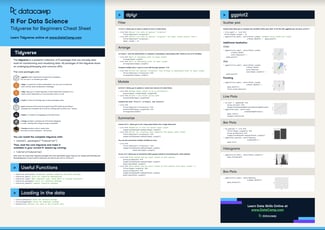
ściągawka
 Karlijn Willems• 7 min
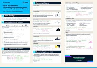
ściągawka
 Richie Cotton

Samouczek
 DataCamp Team• 6 min



Data visualization skills are table stakes for anyone looking to grow their R skills. ggplot2 is one of R’s premiere packages, as it allows an accessible approach to building robust data visualizations in R. In this cheat sheet, you’ll have a handy guide for all the functions and techniques to get you started with ggplot2.