A line plot is a relational data visualization showing how one continuous variable changes when another does. It's one of the most common graphs widely used in finance, sales, marketing, healthcare, natural sciences, and more.
In this tutorial, we'll discuss how to use Seaborn, a popular Python data visualization library, to create and customize line plots in Python.
Introducing the Dataset
To have something to practice seaborn line plots on, we'll first download a Kaggle dataset called Daily Exchange Rates per Euro 1999-2024. Then, we'll import all the necessary packages and read in and clean the dataframe. Without getting into details of the cleaning process, the code below demonstrates the steps to perform:
Currencies:['Australian dollar''Canadian dollar''US dollar']
Date Currency Euro rate
02023-01-27 Australian dollar 1.528912023-01-26 Australian dollar 1.530822023-01-25 Australian dollar 1.536032023-01-24 Australian dollar 1.547042023-01-23 Australian dollar 1.55292022-12-01/2023-01-27
The resulting dataframe contains daily (business days) Euro rates for Australian, Canadian, and US dollars for the period from 01.12.2022 until 27.01.2023 inclusive.
Now, we're ready to dive into creating and customizing Python seaborn line plots.
Seaborn Line Plot Basics
To create a line plot in Seaborn, we can use one of the two functions: lineplot() or relplot(). Overall, they have a lot of functionality in common, together with identical parameter names. The main difference is that relplot() allows us to create line plots with multiple lines on different facets. Instead, lineplot() allows working with confidence intervals and data aggregation.
In this tutorial, we'll mostly use the lineplot() function.
We can create a line plot showing the relationships between two continuous variables as follows:
usd = daily_exchange_rate_df[daily_exchange_rate_df['Currency']=='US dollar'].reset_index(drop=True)
sns.lineplot(x='Date', y='Euro rate', data=usd)Funcționează cu
Output:
The above graph shows the EUR-USD rate dynamics. We defined the variables to plot on the x and y axes (the x and y parameters) and the dataframe (data) to take these variables from.
For comparison, to create the same plot using relplot(), we would write the following:
In this case, we passed in one more argument specific to the relplot() function: kind='line'. By default, this function creates a scatter plot.
Customizing a single seaborn line plot
We can customize the above chart in many ways to make it more readable and informative. For example, we can adjust the figure size, add title and axis labels, adjust the font size, customize the line, add and customize markers, etc. Let's see how to implement these improvements in seaborn.
Adjusting the figure size
Since Seaborn is built on top of matplotlib, we can use matplotlib.pyplot to adjust the figure size:
To add a graph title and axis labels, we can use the set() function on the seaborn line plot object passing in the title, xlabel, and ylabel arguments:
Adding markers and customizing their color, style, and size
It's possible to add markers on the line and customize their appearance. Also, in this case, we can use some parameters from matplotlib, such as marker, markerfacecolor, or markersize:
The documentation provides us with the ultimate list of the parameters to use for improving the aesthetics of a seaborn line plot. In particular, we can see all the possible choices of markers.
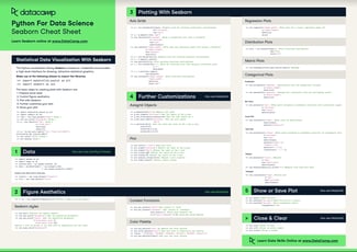
In our Seaborn cheat sheet, you'll find other ways to customize a line plot in Seaborn.
Seaborn Line Plots With Multiple Lines
Often, we need to explore how several continuous variables change depending on another continuous variable. For this purpose, we can build a seaborn line plot with multiple lines. The functions lineplot() and relplot() are also applicable to such cases.
Creating a seaborn line plot with multiple lines
Technically, it's possible to create a seaborn line plot with multiple lines just by building a separate axes object for each dependent variable, i.e., each line:
Above, we extracted two more subsets from our initial dataframe daily_exchange_rate_df – for Australian and Canadian dollars – and plotted each euro rate against time. However, there are more efficient solutions to it: using the hue, style, or size parameters, available in both lineplot() and relplot().
Using the hue parameter
This parameter works as follows: we assign to it the name of a dataframe column containing categorical values, and then seaborn generates a line plot for each category, giving a different color to each line:
sns.lineplot(x='Date', y='Euro rate', data=daily_exchange_rate_df, hue='Currency')Funcționează cu
Output:
With just one line of simple code, we created a seaborn line plot for three categories. Note that we passed in the initial dataframe daily_exchange_rate_df instead of its subsets for different currencies.
Using the style parameter
The style parameter works in the same way as hue, only that it distinguishes between the categories by using different line styles (solid, dashed, dotted, etc.), without affecting the color:
sns.lineplot(x='Date', y='Euro rate', data=daily_exchange_rate_df, style='Currency')Funcționează cu
Output:
Using the size parameter
Just like hue and style, the size parameter creates a separate line for each category. It doesn't affect the color and style of the lines but makes each of them of different width:
sns.lineplot(x='Date', y='Euro rate', data=daily_exchange_rate_df, size='Currency')Funcționează cu
Output:
Customizing a seaborn line plot with multiple lines
Let's now experiment with the aesthetics of our graph. Some techniques here are identical to those we applied to a single Seaborn line plot. The others are specific only to line plots with multiple lines.
Overall adjustments
We can adjust the figure size, add a title and axis labels, and change the font size of the above graph in the same way as we did for a single line plot:
fig = plt.subplots(figsize=(20,5))
sns.lineplot(x='Date', y='Euro rate', data=daily_exchange_rate_df, hue='Currency').set(title='Euro rates for different currencies', xlabel='Date', ylabel='Rate')
sns.set_theme(style='white', font_scale=3)Funcționează cu
Output:
Changing the color, style, and size of each line
Earlier, we saw that when the hue, style, or size parameters are used, seaborn provides a default set of colors/styles/sizes for a line plot with multiple lines. If necessary, we can override these defaults and select colors/styles/sizes by ourselves.
When we use the hue parameter, we can also pass in the palette argument as a list or tuple of matplotlib color names. I would read our tutorial, Seaborn Color Palette: Quick Guide to Picking Colors, to understand more about color theory and to get lots of good ideas to make your visuals look nice.
fig = plt.subplots(figsize=(20,5))
sns.lineplot(x='Date', y='Euro rate', data=daily_exchange_rate_df, hue='Currency', palette=['magenta','deepskyblue','yellowgreen']).set(title='Euro rates for different currencies', xlabel='Date', ylabel='Rate')
sns.set_theme(style='white', font_scale=3)Funcționează cu
Output:
It's also possible to apply directly an existing matplotlib palette:
fig = plt.subplots(figsize=(20,5))
sns.lineplot(x='Date', y='Euro rate', data=daily_exchange_rate_df, hue='Currency', palette='spring').set(title='Euro rates for different currencies', xlabel='Date', ylabel='Rate')
sns.set_theme(style='white', font_scale=3)Funcționează cu
Output:
At the same time, when using hue, we can still adjust the line style and width of all the lines passing in the arguments linestyle and linewidth:
fig = plt.subplots(figsize=(20,5))
sns.lineplot(x='Date', y='Euro rate', data=daily_exchange_rate_df, hue='Currency', palette=['magenta','deepskyblue','yellowgreen'], linestyle='dashed', linewidth=5).set(title='Euro rates for different currencies', xlabel='Date', ylabel='Rate')
sns.set_theme(style='white', font_scale=3)Funcționează cu
Output:
Instead, when we create a seaborn line plot with multiple lines using the style parameter, we can assign a list (or a tuple) of lists (or tuples) to a parameter called dashes:
fig = plt.subplots(figsize=(20,5))
sns.lineplot(x='Date', y='Euro rate', data=daily_exchange_rate_df, style='Currency', dashes=[[4,4],[6,1],[3,9]]).set(title='Euro rates for different currencies', xlabel='Date', ylabel='Rate')
sns.set_theme(style='white', font_scale=3)Funcționează cu
Output:
In the above list of lists assigned to dashes, the first item of each sublist represents the length of a segment of the corresponding line, while the second item – the length of a gap.
Note: to represent a solid line, we need to set the length of a gap to zero, e.g.: [1, 0].
To adjust the color and width of all the lines of this graph, we provide the arguments color and linewidth, just like we did when customizing a single seaborn line plot:
fig = plt.subplots(figsize=(20,5))
sns.lineplot(x='Date', y='Euro rate', data=daily_exchange_rate_df, style='Currency', dashes=[[4,4],[6,1],[3,9]], color='darkviolet', linewidth=4).set(title='Euro rates for different currencies', xlabel='Date', ylabel='Rate')
sns.set_theme(style='white', font_scale=3)Funcționează cu
Output:
Finally, when we use the size parameter to create a seaborn multiple line plot, we can regulate the width of each line through the sizes parameter. It takes in a list (or a tuple) of integers:
fig = plt.subplots(figsize=(20,5))
sns.lineplot(x='Date', y='Euro rate', data=daily_exchange_rate_df, size='Currency', sizes=[2,10,5]).set(title='Euro rates for different currencies', xlabel='Date', ylabel='Rate')
sns.set_theme(style='white', font_scale=3)Funcționează cu
Output:
To customize the color and style of all the lines of this plot, we need to provide the arguments linestyle and color:
fig = plt.subplots(figsize=(20,5))
sns.lineplot(x='Date', y='Euro rate', data=daily_exchange_rate_df, size='Currency', sizes=[2,10,5], linestyle='dotted', color='teal').set(title='Euro rates for different currencies', xlabel='Date', ylabel='Rate')
sns.set_theme(style='white', font_scale=3)Funcționează cu
Output:
Adding markers and customizing their color, style, and size
We may want to add markers on our seaborn multiple line plot.
To add markers of the same color, style, and size on all the lines, we need to use the parameters from matplotlib, such as marker, markerfacecolor, markersize, etc., just as we did for a single line plot:
fig = plt.subplots(figsize=(20,5))
sns.lineplot(x='Date', y='Euro rate', data=daily_exchange_rate_df, hue='Currency', marker='o', markerfacecolor='orangered', markersize=10).set(title='Euro rates for different currencies', xlabel='Date', ylabel='Rate')
sns.set_theme(style='white', font_scale=3)Funcționează cu
Output:
Things are different, though, when we want different markers for each line. In this case, we need to use the markers parameter, which, however, according to seaborn functionalities, works only when the style parameter is specified:
fig = plt.subplots(figsize=(20,5))
sns.lineplot(x='Date', y='Euro rate', data=daily_exchange_rate_df, style='Currency', markers=['o','X','*'], markerfacecolor='brown', markersize=10).set(title='Euro rates for different currencies', xlabel='Date', ylabel='Rate')
sns.set_theme(style='white', font_scale=3)Funcționează cu
Output:
On the above plot, we can make all the lines solid by providing the dashes argument and setting the [1, 0] style pattern to each line:
fig = plt.subplots(figsize=(20,5))
sns.lineplot(x='Date', y='Euro rate', data=daily_exchange_rate_df, style='Currency', markers=['o','X','*'], dashes=[[1,0],[1,0],[1,0]], markerfacecolor='brown', markersize=10).set(title='Euro rates for different currencies', xlabel='Date', ylabel='Rate')
sns.set_theme(style='white', font_scale=3)Funcționează cu
Output:
Conclusion
To recap, in this tutorial, we learned a range of ways to create and customize a Seaborn line plot with either a single or multiple lines.
As a way forward, with seaborn, we can do much more to further adjust a line plot. For example, we can:
Group lines by more than one categorical variable
Customize the legend
Create line plots with multiple lines on different facets
Display and customize the confidence interval
Customize time axis ticks and their labels for a time series line plot
A line plot is a type of plot in Seaborn that shows the relationship between two variables by connecting the data points with a straight line.
What kind of data is best suited for a line plot in Seaborn?⌄
Line plots are best suited for data where there is a clear relationship between two variables, and where the variables are continuous or ordinal.
Can I plot multiple lines on the same plot in Seaborn?⌄
Yes, you can plot multiple lines on the same plot in Seaborn by using the hue parameter to specify a categorical variable to group the data by.
What is the difference between a line plot and a scatter plot in Seaborn?⌄
A line plot in Seaborn shows the relationship between two variables with a straight line, while a scatter plot shows the relationship with individual data points.
Can I add a regression line to my line plot in Seaborn?⌄
Yes, you can add a regression line to your line plot in Seaborn by using the regplot() function, which fits and plots a linear regression model between two variables.
How do I save my Seaborn line plot to a file?⌄
You can save your Seaborn line plot to a file by using the savefig() function from the matplotlib library, which saves the current figure to a specified file path and format.
Learn to create and customize Seaborn barplots in Python. Master essential techniques for visualizing categorical data relationships, from basic plots to advanced features.







A line plot is a relational data visualization showing how one continuous variable changes when another does. It's one of the most common graphs widely used in finance, sales, marketing, healthcare, natural sciences, and more.
In this tutorial, we'll discuss how to use Seaborn, a popular Python data visualization library, to create and customize line plots in Python.
Introducing the Dataset
To have something to practice seaborn line plots on, we'll first download a Kaggle dataset called Daily Exchange Rates per Euro 1999-2024. Then, we'll import all the necessary packages and read in and clean the dataframe. Without getting into details of the cleaning process, the code below demonstrates the steps to perform:
Output:
The resulting dataframe contains daily (business days) Euro rates for Australian, Canadian, and US dollars for the period from
01.12.2022until27.01.2023inclusive.Now, we're ready to dive into creating and customizing Python seaborn line plots.
Seaborn Line Plot Basics
To create a line plot in Seaborn, we can use one of the two functions:
lineplot()orrelplot(). Overall, they have a lot of functionality in common, together with identical parameter names. The main difference is thatrelplot()allows us to create line plots with multiple lines on different facets. Instead,lineplot()allows working with confidence intervals and data aggregation.In this tutorial, we'll mostly use the
lineplot()function.The course Introduction to Data Visualization with Seaborn will help you learn and practice the main functions and methods of the seaborn library. You can also check out our Seaborn tutorial for beginners to get more familiar with the popular Python library.
Creating a single seaborn line plot
We can create a line plot showing the relationships between two continuous variables as follows:
Output:
The above graph shows the EUR-USD rate dynamics. We defined the variables to plot on the x and y axes (the x and y parameters) and the dataframe (data) to take these variables from.
For comparison, to create the same plot using
relplot(), we would write the following:Output:
In this case, we passed in one more argument specific to the
relplot()function:kind='line'. By default, this function creates a scatter plot.Customizing a single seaborn line plot
We can customize the above chart in many ways to make it more readable and informative. For example, we can adjust the figure size, add title and axis labels, adjust the font size, customize the line, add and customize markers, etc. Let's see how to implement these improvements in seaborn.
Adjusting the figure size
Since Seaborn is built on top of matplotlib, we can use
matplotlib.pyplotto adjust the figure size:Output:
Instead, with relplot(), we can use the height and aspect (the width-to-height ratio) parameters for the same purpose:
Output:
Adding a title and axis labels
To add a graph title and axis labels, we can use the
set()function on the seaborn line plot object passing in the title,xlabel, andylabelarguments:Output:
Adjusting the font size
A convenient way to adjust the font size is to use the
set_theme()function and experiment with different values of thefont_scaleparameter:Output:
Note that we also added
style='white'to avoid overriding the initial style.Changing the line color, style, and size
To customize the plot line, we can pass in some optional parameters in common with
matplotlib.pyplot.plot, such ascolor,linestyle, orlinewidth:Output:
Adding markers and customizing their color, style, and size
It's possible to add markers on the line and customize their appearance. Also, in this case, we can use some parameters from matplotlib, such as
marker,markerfacecolor, ormarkersize:Output:
The documentation provides us with the ultimate list of the parameters to use for improving the aesthetics of a seaborn line plot. In particular, we can see all the possible choices of markers.
In our Seaborn cheat sheet, you'll find other ways to customize a line plot in Seaborn.
Seaborn Line Plots With Multiple Lines
Often, we need to explore how several continuous variables change depending on another continuous variable. For this purpose, we can build a seaborn line plot with multiple lines. The functions
lineplot()andrelplot()are also applicable to such cases.Creating a seaborn line plot with multiple lines
Technically, it's possible to create a seaborn line plot with multiple lines just by building a separate axes object for each dependent variable, i.e., each line:
Output:
Above, we extracted two more subsets from our initial dataframe
daily_exchange_rate_df– for Australian and Canadian dollars – and plotted each euro rate against time. However, there are more efficient solutions to it: using thehue,style, orsizeparameters, available in bothlineplot()andrelplot().Using the hue parameter
This parameter works as follows: we assign to it the name of a dataframe column containing categorical values, and then seaborn generates a line plot for each category, giving a different color to each line:
Output:
With just one line of simple code, we created a seaborn line plot for three categories. Note that we passed in the initial dataframe
daily_exchange_rate_dfinstead of its subsets for different currencies.Using the style parameter
The style parameter works in the same way as hue, only that it distinguishes between the categories by using different line styles (solid, dashed, dotted, etc.), without affecting the color:
Output:
Using the size parameter
Just like hue and style, the size parameter creates a separate line for each category. It doesn't affect the color and style of the lines but makes each of them of different width:
Output:
Customizing a seaborn line plot with multiple lines
Let's now experiment with the aesthetics of our graph. Some techniques here are identical to those we applied to a single Seaborn line plot. The others are specific only to line plots with multiple lines.
Overall adjustments
We can adjust the figure size, add a title and axis labels, and change the font size of the above graph in the same way as we did for a single line plot:
Output:
Changing the color, style, and size of each line
Earlier, we saw that when the hue, style, or size parameters are used, seaborn provides a default set of colors/styles/sizes for a line plot with multiple lines. If necessary, we can override these defaults and select colors/styles/sizes by ourselves.
When we use the hue parameter, we can also pass in the
paletteargument as a list or tuple of matplotlib color names. I would read our tutorial, Seaborn Color Palette: Quick Guide to Picking Colors, to understand more about color theory and to get lots of good ideas to make your visuals look nice.Output:
It's also possible to apply directly an existing matplotlib palette:
Output:
At the same time, when using
hue, we can still adjust the line style and width of all the lines passing in the argumentslinestyleandlinewidth:Output:
Instead, when we create a seaborn line plot with multiple lines using the style parameter, we can assign a list (or a tuple) of lists (or tuples) to a parameter called dashes:
Output:
In the above list of lists assigned to dashes, the first item of each sublist represents the length of a segment of the corresponding line, while the second item – the length of a gap.
Note: to represent a solid line, we need to set the length of a gap to zero, e.g.:
[1, 0].To adjust the color and width of all the lines of this graph, we provide the arguments color and linewidth, just like we did when customizing a single seaborn line plot:
Output:
Finally, when we use the size parameter to create a seaborn multiple line plot, we can regulate the width of each line through the
sizesparameter. It takes in a list (or a tuple) of integers:Output:
To customize the color and style of all the lines of this plot, we need to provide the arguments linestyle and color:
Output:
Adding markers and customizing their color, style, and size
We may want to add markers on our seaborn multiple line plot.
To add markers of the same color, style, and size on all the lines, we need to use the parameters from matplotlib, such as marker,
markerfacecolor,markersize, etc., just as we did for a single line plot:Output:
Things are different, though, when we want different markers for each line. In this case, we need to use the markers parameter, which, however, according to seaborn functionalities, works only when the style parameter is specified:
Output:
On the above plot, we can make all the lines solid by providing the dashes argument and setting the
[1, 0]style pattern to each line:Output:
Conclusion
To recap, in this tutorial, we learned a range of ways to create and customize a Seaborn line plot with either a single or multiple lines.
As a way forward, with seaborn, we can do much more to further adjust a line plot. For example, we can:
To dig deeper into what and how can be done with seaborn, consider taking our course Intermediate Data Visualization with Seaborn.