使用 Python 在 Matplotlib 中绘制折线图

在 Matplotlib 中创建基础折线图

我们先创建一个基础折线图，然后再进行美化和信息增补，使图表更美观、更有信息量。

使用 plt.plot() 创建折线图

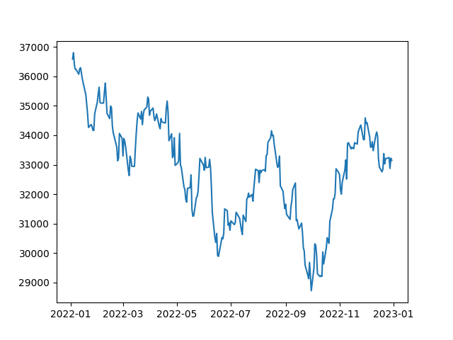
创建折线图时，我们使用 plt.plot() 函数。该函数接收两个参数：x 轴取值与 y 轴取值。在这里，日期列将作为 x 轴，收盘价列作为 y 轴。示例代码如下：

# Extract the date and close price columns
dates = df['Date']
closing_price = df['Close']

# Create a line plot
plt.plot(dates, closing_price)

# Show the plot
plt.show()技术支持

运行上述代码后，您将看到 DJIA 股价的基础折线图。

自定义折线图

Matplotlib 提供了丰富的自定义选项，您可以按需灵活调整。

设置线条颜色

默认情况下，plt.plot() 绘制的是蓝色线条。您可以通过传入 color 参数更改颜色。color 参数可以接收颜色名字符串或十六进制颜色代码。

示例如下：

# Plot in Red colour
plt.plot(dates, closing_price, color='red')

# Show the plot
plt.show()技术支持

这段代码会将默认的蓝色线条改为红色，如下图所示：

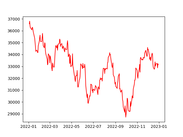
红色的基础折线图

设置线条宽度

您还可以通过向 plt.plot() 传入 linewidth 参数来更改线宽。linewidth 参数接收浮点数，表示线条的宽度。

示例如下：

# Increasing the linewidth
plt.plot(dates, closing_price, linewidth=3)

# Show the plot
plt.show()技术支持

这段代码会将线宽设置为 3，高于默认值，如下图所示：

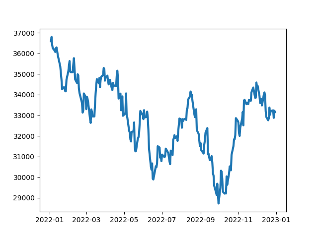
更高的 linewidth 带来更粗的线条

设置线条样式

您可以通过向 plt.plot() 传入 linestyle 参数来更改线型。linestyle 接收表示线型的字符串。Matplotlib 文档提供了详尽的可用样式列表。

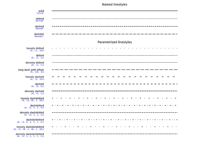
以下是这些样式在代码中的用法：

# Individually plot lines in solid, dotted, dashed and dashdot

plt.plot(dates, closing_price, linestyle='solid') # Default line style
plt.plot(dates, closing_price, linestyle='dotted')
plt.plot(dates, closing_price, linestyle='dashed')
plt.plot(dates, closing_price, linestyle='dashdot')

# Show the plot
plt.show()技术支持

为折线图添加标记

标记可用于突出显示折线图中的特定点。可以使用多种符号作为标记，完整列表参见Matplotlib 文档。

以下是在折线图中使用标记的示例：

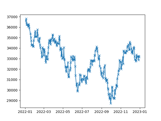
# Add a cross marker for each point
plt.plot(df['Date'], df['Close'], marker='x')

# Show the plot
plt.show()技术支持

在上述代码中，我们使用叉号（x）标记来突出显示 DJIA 的 Close 价格，如下图所示：

添加坐标轴标签和标题

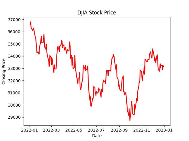
为了让图表更具信息性，我们可以添加坐标轴标签与标题。分别使用 plt.xlabel()、plt.ylabel() 和 plt.title() 即可实现。

示例如下：

plt.plot(dates, closing_price, color='red', linewidth=2)
plt.xlabel('Date')
plt.ylabel('Closing Price')
plt.title('DJIA Stock Price')

# Show the plot
plt.show()技术支持

这段代码会绘制一条线宽为 2 的红色折线，同时为 x 轴添加“Date”、y 轴添加“Closing Price”，并设置标题为“DJIA Stock Price”。

添加网格线

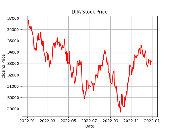
我们也可以为图表添加网格线以提升可读性。使用 plt.grid() 函数即可。该函数接收布尔值，用于控制是否显示网格。

示例如下：

plt.plot(dates, closing_price, color='red', linewidth=2)
plt.xlabel('Date')
plt.ylabel('Closing Price')
plt.title('DJIA Stock Price')

# Add the grid
plt.grid(True)

# Show the plot
plt.show()技术支持

您会看到图表中增加了网格：

包含多条线的 Matplotlib 折线图

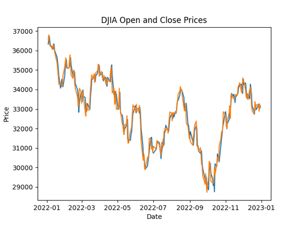
在某些情况下，您可能希望在同一张图上绘制多条折线。此时可以多次调用 plt.plot()，每次传入不同的数据。示例如下：

# Line plot of Open and Close prices

plt.plot(df['Date'], df['Open'])
plt.plot(df['Date'], df['Close'])
plt.title('DJIA Open and Close Prices')
plt.xlabel('Date')
plt.ylabel('Price')

plt.show()技术支持

在上述代码中，我们在同一图中绘制了 DJIA 的 Open 与 Close 价格。

带双坐标轴的 Matplotlib 折线图

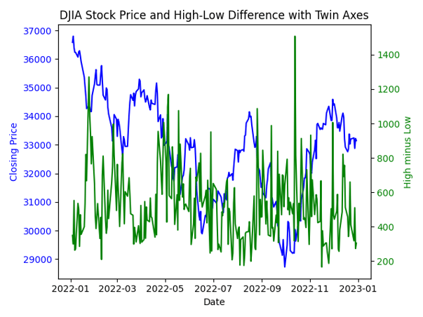
有时您需要在同一张图中展示两个量纲不同的变量。此类场景下，使用双坐标轴可以在不牺牲各自刻度清晰度的前提下，直观展现二者之间的关系。

要创建带双坐标轴的折线图，我们需要使用 twinx() 函数。该函数会创建一个与原图共享 x 轴的新 y 轴。

示例如下：

# Create a new variable for demonstration purposes
df['High_minus_Low'] = df['High'] - df['Low']

# Create a basic line plot for the Close prices
fig, ax1 = plt.subplots()
ax1.plot(df['Date'], df['Close'], color='blue', label='Close Price')
ax1.set_xlabel('Date')
ax1.set_ylabel('Closing Price', color='blue')
ax1.tick_params(axis='y', labelcolor='blue')

# Create a twin axis for the High_minus_Low variable
ax2 = ax1.twinx()
ax2.plot(df['Date'], df['High_minus_Low'], color='green', label='High - Low')
ax2.set_ylabel('High minus Low', color='green')
ax2.tick_params(axis='y', labelcolor='green')

# Add a title and show the plot
plt.title('DJIA Stock Price and High-Low Difference with Twin Axes')
plt.show()技术支持

生成的双坐标轴图如下：

在 Matplotlib 折线图中添加统计信息

除了用来展示数据的趋势和模式，折线图还可以叠加统计信息，如回归线与误差线。

添加 Matplotlib 回归线

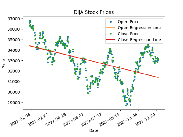
回归线是在图中最能拟合数据点的直线，可用于建模与预测未来值。我们可以使用 NumPy 的 polyfit() 函数将多项式回归线拟合到数据点上，并将其添加到折线图中。

import matplotlib.dates as mdates

# Convert Date column to numeric value
df['Date'] = mdates.date2num(df['Date'])

# Add regression line to plot
coefficients_open = np.polyfit(df['Date'], df['Open'], 1)
p_open = np.poly1d(coefficients_open)

coefficients_close = np.polyfit(df['Date'], df['Close'], 1)
p_close = np.poly1d(coefficients_close)

fig, ax = plt.subplots()
ax.plot(df['Date'], df['Open'], '.', label='Open Price')
ax.plot(df['Date'], p_open(df['Date']), '-', label='Open Regression Line')
ax.plot(df['Date'], df['Close'], '.', label='Close Price')
ax.plot(df['Date'], p_close(df['Date']), '-', label='Close Regression Line')
ax.set_title('DIJA Stock Prices')
ax.set_xlabel('Date')
ax.set_ylabel('Price')
ax.legend()

# Format x-axis labels as dates
date_form = mdates.DateFormatter("%Y-%m-%d")
ax.xaxis.set_major_formatter(date_form)
plt.gcf().autofmt_xdate()

plt.show()技术支持

在这段代码中，我们首先使用 date2num() 函数将日期转换为数值，然后使用 polyfit() 函数求得回归线的系数。接着用 poly1d() 函数构造回归线并进行绘制。原始数据点以散点表示，回归线以实线表示。

添加误差线

误差线是对数据变异性的图形化表征，可用于表示测量中的不确定性。

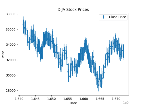
当您预计数据采集过程中会有误差时（如气温数据、空气质量数据等），这尤其有用。尽管股价数据相对确定，这里我们假设存在一个标准差量级的潜在误差，并使用 Matplotlib 的 errorbar 函数将其绘制出来。

# Calculate standard deviation of data
std = df['Close'].std()

# Add error bars to plot
plt.errorbar(df['Date'], df['Close'], yerr=std/2, fmt='.', label='Close Price')
plt.title('DIJA Stock Prices')
plt.xlabel('Date')
plt.ylabel('Price')
plt.legend()
plt.show()技术支持

在这段代码中，我们首先计算数据集中 Close 价格的标准差。随后使用 errorbar() 函数为折线图添加误差线，误差大小设为标准差的一半。

通过这些技巧，我们可以在折线图中加入统计信息，从而更深入地洞察数据。

结语

折线图是可视化数据趋势与模式的有力工具，而 Matplotlib 提供了易用的接口来创建这类图表。

下一步，您可以继续学习我们的Intermediate Python 课程，在其中把学到的内容应用到黑客统计学的案例研究中。

我们希望本教程能帮助您顺利上手在 Matplotlib 中创建折线图。我们还在另一篇教程中对其他Matplotlib 图表进行了系统讲解，能帮助您快速了解 Matplotlib 的更多用法。

继续探索与尝试，打造精彩的可视化，并从数据中发掘更多洞见！