Curso
Python intermedio
4 h
1.4M
Most of you are familiar with image data, taken with ordinary cameras (these are often called “natural images” in the scientific literature), but also with specialized instruments, such as microscopes or telescopes. When working with images in Python, the most common way to display them is using the imshow function of Matplotlib, Python’s most popular plotting library.
In this tutorial, we’ll show you how to extend this function to display 3D volumetric data, which you can think of as a stack of images. Together, they describe a 3D structure. For example, magnetic resonance imaging (MRI) and computed tomography (CT) scans measure the 3D structure inside the human body; X-ray microtomography measures the 3D structure inside materials such as glass, or metal alloys; and light-sheet microscopes measure fluorescent particles inside biological tissues.
We’ll demonstrate how to download an MRI dataset and display the slices using matplotlib. You’ll learn how to
nibabel library, which provides a reader for files with the NIfTI file format. For those of you who might want to skip this step and directly start plotting, this tutorial will show you how to get the data with scikit-image.But first, let’s go over some basics: how to display images with Matplotlib’s imshow.
You can start by enabling the interactive matplotlib mode if you’re working with Jupyter Notebook:
%matplotlib notebookNow you can import matplotlib and display some data. You’ll load some example data that is included in the data module of the scikit-image library:
import matplotlib.pyplot as plt
from skimage import data

astronaut = data.astronaut()
ihc = data.immunohistochemistry()
hubble = data.hubble_deep_field()

# Initialize the subplot panels side by side
fig, ax = plt.subplots(nrows=1, ncols=3)

# Show an image in each subplot
ax[0].imshow(astronaut)
ax[0].set_title('Natural image')
ax[1].imshow(ihc)
ax[1].set_title('Microscopy image')
ax[2].imshow(hubble)
ax[2].set_title('Telescope image');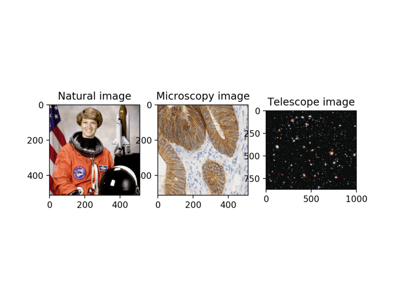
Note: When you run matplotlib in the interactive notebook mode, the open figure remains the only active figure until you disable it, using the power symbol on the top-right of the figure. Be sure you do that before moving on from each plot.
These images are called 2-dimensional or 2D images because they are laid out along 2 dimensions: x and y, or, in NumPy parlance, rows and columns or r and c.
Some images are 3D, in that they have an additional depth dimension (z, or planes). These include magnetic resonance imaging (MRI) and serial section transmission electron microscopy (ssTEM), in which a sample is thinly sliced, like a salami, and each of the slices is imaged separately.
To view such images in matplotlib, we have to choose a slice, and display only that slice. Let’s try it out on some freely available MRI data online.
We’re going to download a dataset described in Buchel and Friston, Cortical Interactions Evaluated with Structural Equation Modelling and fMRI (1997). First, we create a temporary directory in which to download the data. We must remember to delete it when we are done with our analysis! If you want to keep this dataset for later use, change d to a more permanent directory location of your choice.
import tempfile

# Create a temporary directory
d = tempfile.mkdtemp()
Now, let’s download the data:
import os

# Return the tail of the path
os.path.basename('http://google.com/attention.zip')
from urllib.request import urlretrieve
# Define URL
url = 'http://www.fil.ion.ucl.ac.uk/spm/download/data/attention/attention.zip'
# Retrieve the data
fn, info = urlretrieve(url, os.path.join(d, 'attention.zip'))And extract it from the zip file to our temporary directory:
import zipfile

# Extract the contents into the temporary directory we created earlier
zipfile.ZipFile(fn).extractall(path=d)
If you look at the actual contents of the file, you’ll find a bunch of ‘.hdr’ and ‘.img’ files.
# List first 10 files
[f.filename for f in zipfile.ZipFile(fn).filelist[:10]]
These are in the NIfTI file format, and we’ll need a reader for them. Thankfully, the excellent nibabel library provides such a reader. Make sure you install it with either conda install -c conda-forge nibabel or pip install nibabel, and then:
import nibabelNow, we can finally read our image, and use the .get_data() method to get a NumPy array to view:
# Read the image
struct = nibabel.load(os.path.join(d, 'attention/structural/nsM00587_0002.hdr'))

# Get a plain NumPy array, without all the metadata
struct_arr = struct.get_data()
Tip: if you want to directly continue to plotting the MRI data, execute the following lines of code:
from skimage import io

struct_arr = io.imread("https://s3.amazonaws.com/assets.datacamp.com/blog_assets/attention-mri.tif")Let’s now look at a slice in that array:
plt.imshow(struct_arr[75])
Whoa! That looks pretty squishy! That’s because the resolution along the vertical axis in many MRIs is not the same as along the horizontal axes. We can fix that by passing the aspect parameter to the imshow function:
plt.imshow(struct_arr[75], aspect=0.5)
But, to make things easier, we will just transpose the data and only look at the horizontal slices, which don’t need such fiddling.
struct_arr2 = struct_arr.T
plt.imshow(struct_arr2[34])
Pretty! Of course, to then view another slice, or a slice along a different axis, we need another call to imshow:
plt.imshow(struct_arr2[5])
All these calls get rather tedious rather quickly. For a long time, I would view 3D volumes using tools outside Python, such as ITK-SNAP. But, as it turns out, it’s quite easy to add 3D “scrolling” capabilities to the matplotlib viewer! This lets us explore 3D data within Python, minimizing the need to switch contexts between data exploration and data analysis.
The key is to use the matplotlib event handler API, which lets us define actions to perform on the plot — including changing the plot’s data! — in response to particular key presses or mouse button clicks.
In our case, let’s bind the J and K keys on the keyboard to “previous slice” and “next slice”:
def previous_slice():
    pass

def next_slice():
    pass

def process_key(event):
    if event.key == 'j':
        previous_slice()
    elif event.key == 'k':
        next_slice()
Simple enough! Of course, we need to figure out how to actually implement these actions and we need to tell the figure that it should use the process_key function to process keyboard presses! The latter is simple: we just need to use the figure canvas method mpl_connect:
fig, ax = plt.subplots()
ax.imshow(struct_arr[..., 43])
fig.canvas.mpl_connect('key_press_event', process_key)
You can find the full documentation for mpl_connect here, including what other kinds of events you can bind (such as mouse button clicks).
It took me just a bit of exploring to find out that imshow returns an AxesImage object, which lives “inside” the matplotlib Axes object where all the drawing takes place, in its .images attribute. And this object provides a convenient set_array method that swaps out the image data being displayed! So, all we need to do is:
Axes object.next_slice and previous_slice that change the index and uses set_array to set the corresponding slice of the 3D volume.draw method to redraw the figure with the new data.def multi_slice_viewer(volume):
fig, ax = plt.subplots()
ax.volume = volume
ax.index = volume.shape[0] // 2
ax.imshow(volume[ax.index])
fig.canvas.mpl_connect('key_press_event', process_key)
def process_key(event):
fig = event.canvas.figure
ax = fig.axes[0]
if event.key == 'j':
previous_slice(ax)
elif event.key == 'k':
next_slice(ax)
fig.canvas.draw()
def previous_slice(ax):
"""Go to the previous slice."""
volume = ax.volume
ax.index = (ax.index - 1) % volume.shape[0] # wrap around using %
ax.images[0].set_array(volume[ax.index])
def next_slice(ax):
"""Go to the next slice."""
volume = ax.volume
ax.index = (ax.index + 1) % volume.shape[0]
ax.images[0].set_array(volume[ax.index])Let’s try it out!
multi_slice_viewer(struct_arr2)
This works! Nice! But, if you try this out at home, you’ll notice that scrolling up with K also squishes the horizontal scale of the plot. Huh? (This only happens if your mouse is over the image.)
What’s happening is that adding event handlers to Matplotlib simply piles them on on top of each other. In this case, K is a built-in keyboard shortcut to change the x-axis to use a logarithmic scale. If we want to use K exclusively, we have to remove it from matplotlib’s default key maps. These live as lists in the plt.rcParams dictionary, which is matplotlib’s repository for default system-wide settings:
plt.rcParams['keymap.<command>'] = ['<key1>', '<key2>']where pressing any of the keys in the list (i.e. <key1> or <key2>) will cause <command> to be executed.
Thus, we’ll need to write a helper function to remove keys that we want to use wherever they may appear in this dictionary. (This function doesn’t yet exist in matplotlib, but would probably be a welcome contribution!)
def remove_keymap_conflicts(new_keys_set):
    for prop in plt.rcParams:
        if prop.startswith('keymap.'):
            keys = plt.rcParams[prop]
            remove_list = set(keys) & new_keys_set
            for key in remove_list:
keys.remove(key)Ok, let’s rewrite our function to make use of this new tool:
def multi_slice_viewer(volume):
    remove_keymap_conflicts({'j', 'k'})
    fig, ax = plt.subplots()
    ax.volume = volume
    ax.index = volume.shape[0] // 2
    ax.imshow(volume[ax.index])
    fig.canvas.mpl_connect('key_press_event', process_key)

def process_key(event):
    fig = event.canvas.figure
    ax = fig.axes[0]
    if event.key == 'j':
        previous_slice(ax)
    elif event.key == 'k':
        next_slice(ax)
    fig.canvas.draw()

def previous_slice(ax):
    volume = ax.volume
    ax.index = (ax.index - 1) % volume.shape[0]  # wrap around using %
    ax.images[0].set_array(volume[ax.index])

def next_slice(ax):
    volume = ax.volume
    ax.index = (ax.index + 1) % volume.shape[0]
    ax.images[0].set_array(volume[ax.index])
Now, we should be able to view all the slices in our MRI volume without pesky interference from the default keymap!
multi_slice_viewer(struct_arr2)
One nice feature about this method is that it works on any matplotlib backend! So, if you try this out in the IPython terminal console, you will still get the same interaction as you did in the browser! And the same is true for a Qt or Tkinter app embedding a matplotlib plot. This simple tool therefore lets you build ever more complex applications around matplotlib’s visualization capabilities.
Let’s not forget to clean up after ourselves, and delete the temporary directory (if you made one):
import shutil

# Remove the temporary directory
shutil.rmtree(d)Congrats! It has been quite a journey, but you have made it to the end of this Matplotlib tutorial!
Make sure to stay tuned for the second post of this series, in which you’ll learn more on scaling subplots, crosshairs that show where each plot is sliced, and mouse interactivity.
Check out DataCamp's Matplotlib Tutorial: Python Plotting.
If you want to know more about data visualization in Python, consider taking DataCamp’s Introduction to Data Visualization in Python course.
Learn more about Python
Curso
Curso
Curso
blog
Karlijn Willems
11 min
Tutorial
Kevin Babitz
Tutorial
Aditya Sharma
Tutorial
Elena Kosourova
code-along
Justin Saddlemyer
code-along
Filip Schouwenaars