Excel makes it simple to visualize data, and one of the most effective ways to display trends over time is with a line graph. Whether you're tracking sales, monitoring performance metrics, or analyzing scientific data, a well-designed line graph helps make patterns clear and insights easier to understand.
Manually scanning rows of numbers can be overwhelming, but a line graph turns those numbers into a visual story. With a simple setup, Excel allows you to create a graph that highlights trends, comparisons, and key changes in your data. To maximize its potential, it's crucial to correctly structure your data, select the appropriate settings, and implement customizations that enhance readability.
This guide walks you through every step of the process. You'll start by preparing your data, then create a basic line graph using Excel’s built-in tools. From there, you'll learn how to customize your graph with labels, multiple lines, and formatting options that enhance clarity. By the end, you'll have the skills to create professional-looking graphs that make your data easier to interpret and share.
If you’re still working on your Excel skills, you can gain the essentials, from preparing data to writing formulas and creating visualizations, with our Excel Fundamentals skill track.
Preparing Your Data
Before making a graph, the data needs to be formatted correctly. Each column should have a clear header, and numerical values should be arranged properly. For example, if tracking sales over months, the first column should list the months, while the second column contains the sales figures. Ensuring that numbers are properly entered and labels are clear will help Excel generate an accurate graph.
Example dataset:
Date	Daily Rainfall	Particulate
1/1/2007	4.1	122
1/2/2007	4.3	117
1/3/2007	5.7	112
1/4/2007	5.4	114
1/5/2007	5.9	110
1/6/2007	5	114
1/7/2007	3.6	128
1/8/2007	1.9	137
1/9/2007	7.3	104
Creating a Basic Line Graph in Excel
Once the data is ready, head to the Insert tab and insert a blank line chart. This will create a blank canvas that we can start with.
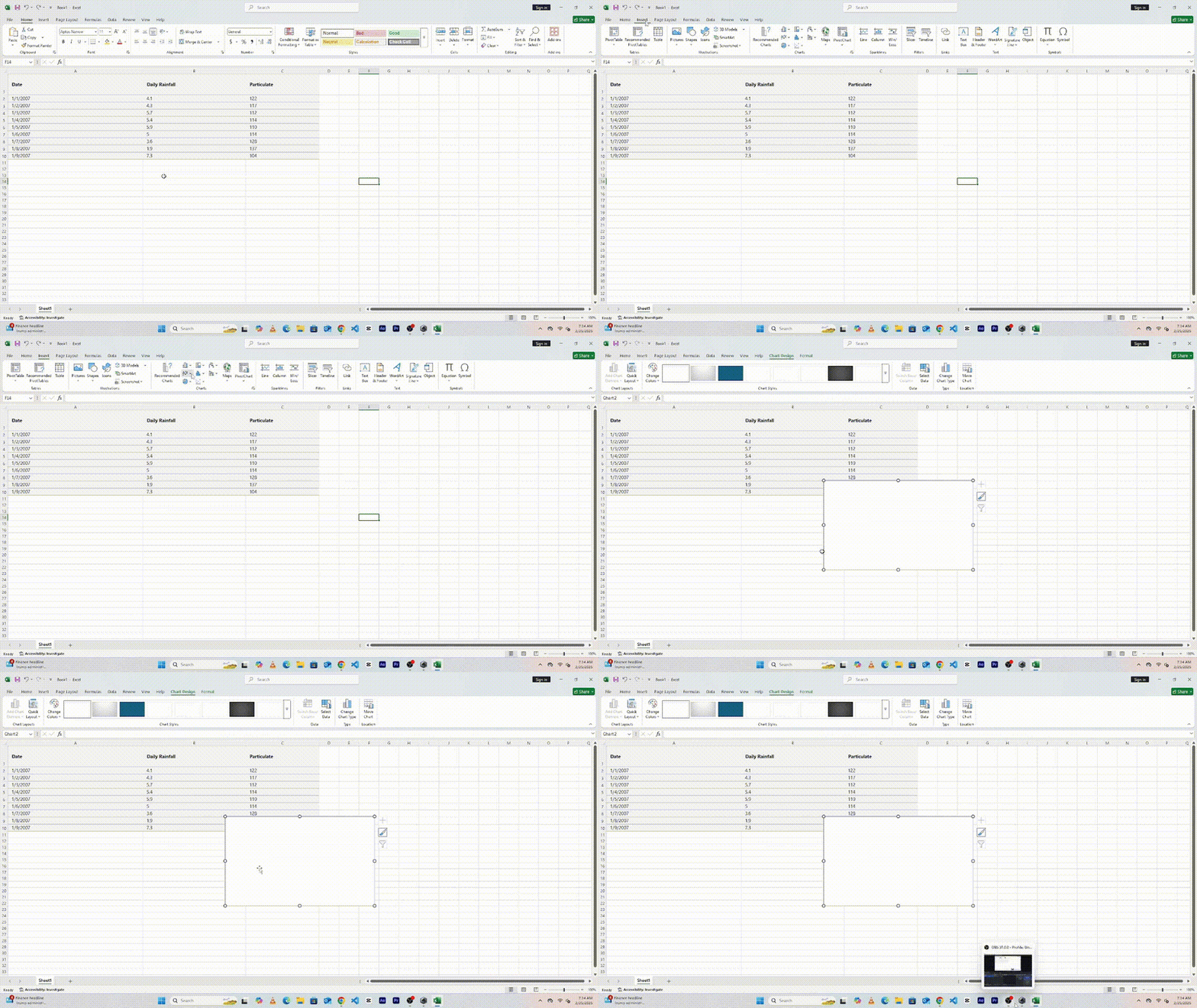
Next, follow these steps to create the line graph:
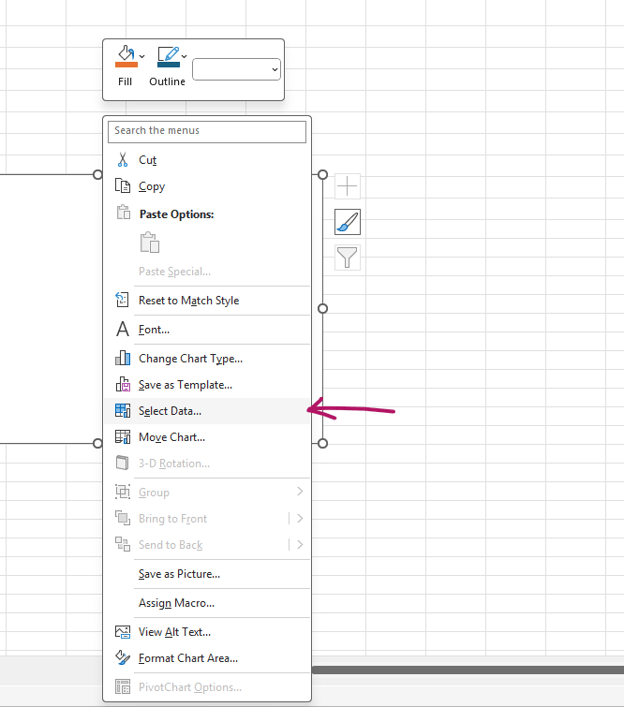
- Right-click on the blank canvas
- Click Select Data
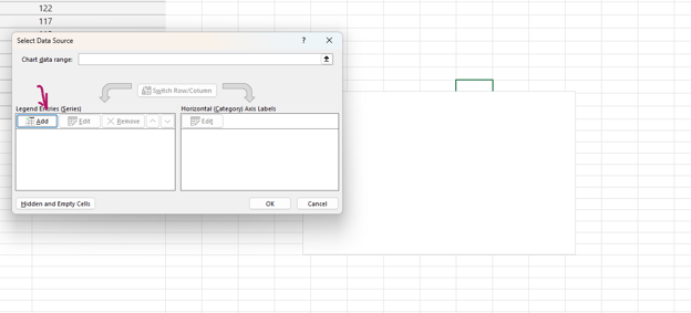
- Click Add
- On the series name, write the name of the quantity column, in this case, Daily Rainfall.
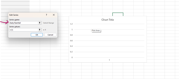
- On the series values, select the range of values in the quantity column that you want to include in the line graph.
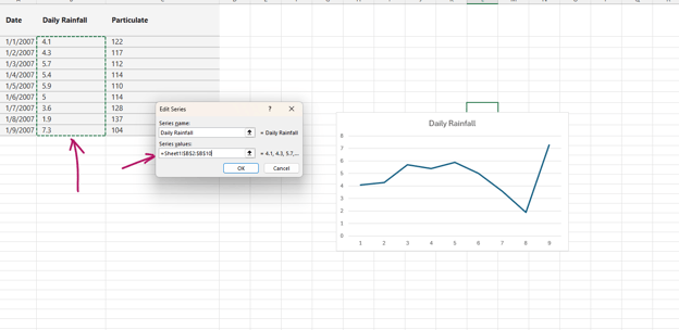
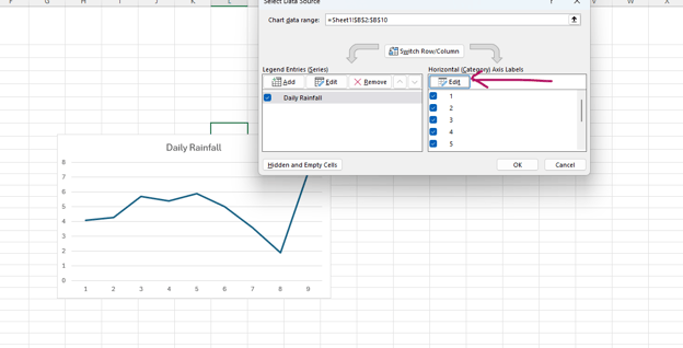
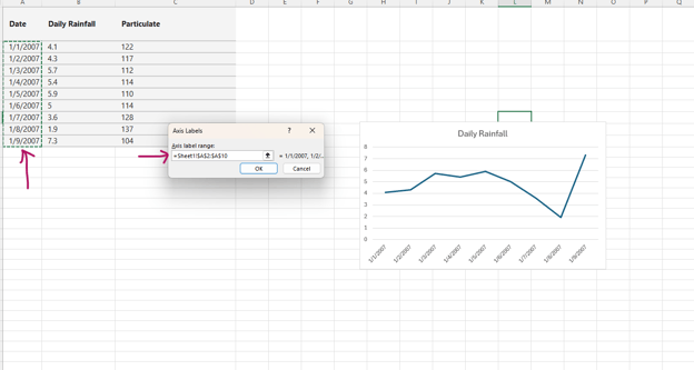
- On the horizontal axis, select the column with the date values, in this case, Date.
- Drag the cells you want to include
Customizing the Excel Line Graph
The next step is refining the graph to communicate the information effectively.
Changing the graph title and labels
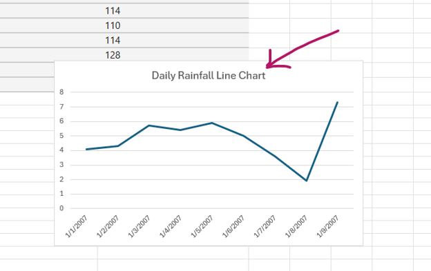
Edit the title to describe what the graph clearly represents. Check and adjust as needed to make the data easier to understand.
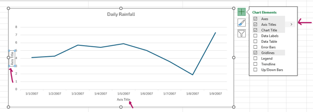
To change the axis labels, click on the graph and press the green plus button. This will allow you to toggle the axis. Once they appear, you can click to modify them.
Switching X and Y axis
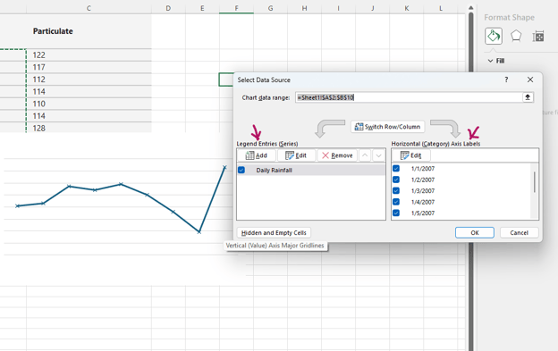
If Excel plots the axes incorrectly, you can switch them using the "Select Data" feature. This ensures that the right values appear on the correct axis.
Adding multiple lines to the graph
If there are multiple datasets to compare, you can add additional lines to the graph. This can be done by selecting more data while creating the chart or by adding a new series through the "Select Data" menu. To differentiate between lines, change colors and styles so that each dataset stands out.
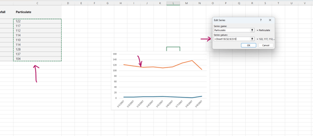
In the example below, we add a new line chart for the Particulate column.
Follow these steps to add a new line:
- Right-click on the chart and choose Select Data.
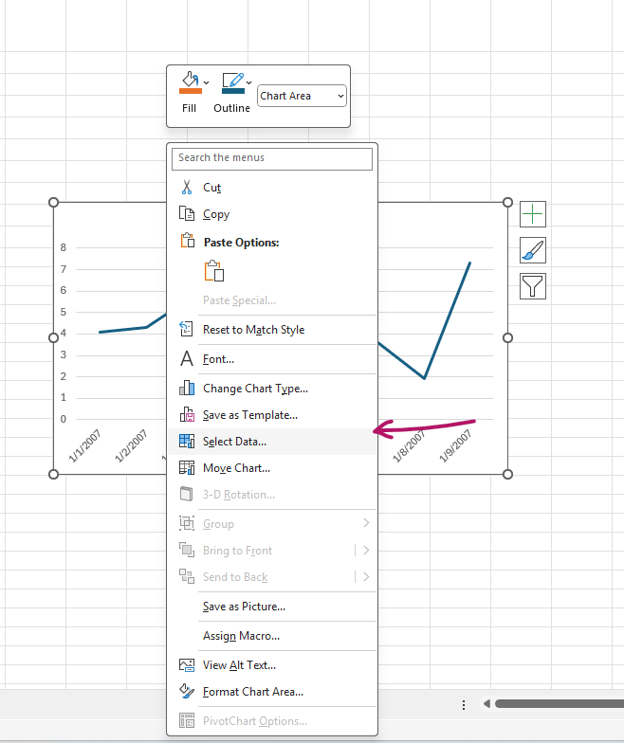
- Click on Add to choose the values for the new column
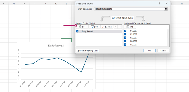
- Add the series name and choose the values for the new column, in this case Particulate.
Changing the graph title and labels
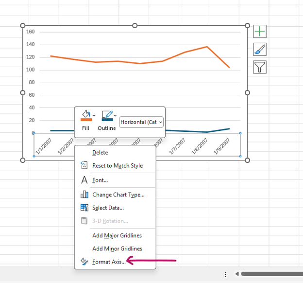
Sometimes, the data on the horizontal axis might be hard to read, especially if you have a lot of data. You can adjust it to make it more readable; for example, you can tilt the axis. To do this, right-click on the axis and press Format Axis.
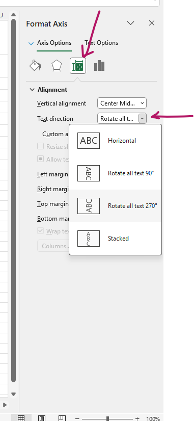
On the Size and Properties menu, choose the desired text direction.
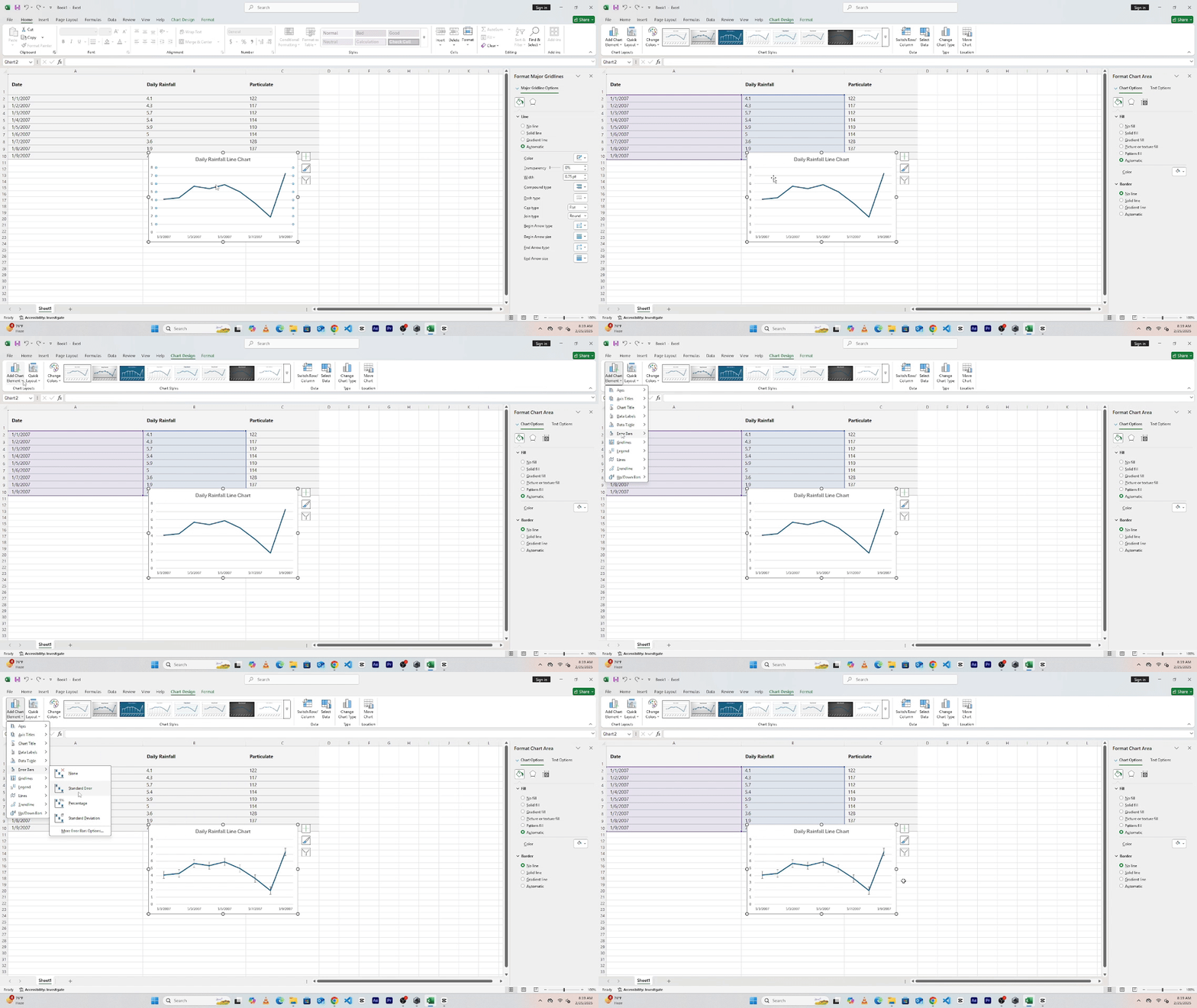
You can also add a vertical line for reference, such as marking an important date. This can be done by using a scatter plot or error bars to place a single point or line at a specific position on the graph.
Adding a vertical line to the graph
For example, to add a standard error bar, double-click on the chart, then on the top left, choose Add Chart Element and choose Standard Error Bar.
Enhancing Excel Line Graphs for Better Visualization
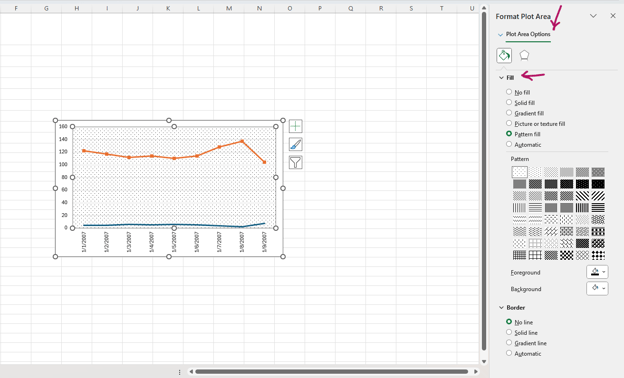
To make the graph more visually appealing and easy to read, you can adjust colors and styles. Different line styles can help separate datasets. For example, you can add markers to highlight data points, making trends easier to follow. You can also modify gridlines and background colors to create a cleaner look that works well in reports and presentations.
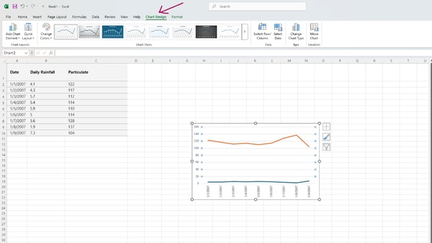
Different line styles can help separate datasets. For example, you can add markers to highlight data points, making trends easier to follow.
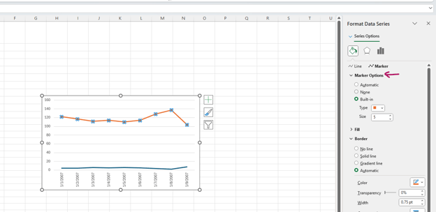
You can also modify gridlines and background colors to create a cleaner look that works well in reports and presentations.
Saving and Exporting the Graph from Excel
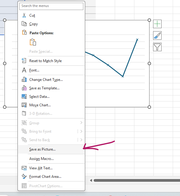
Once the graph is complete, you can save or export it for use in reports or presentations. Excel allows charts to be copied and pasted into other documents. They can also be saved as images or PDFs, making it easy to share the graph with others.
A well-designed line graph helps present data in a way that is easy to understand. By following these steps, you can create clear and professional-looking charts that make trends and patterns stand out.
Conclusion
Throughout this article, we’ve explored how to create a line graph in Excel, from setting up your data to customizing the chart for better readability. By following these steps, you can turn raw numbers into clear visuals that highlight trends and make your data easier to understand.
Whether you’re tracking business performance, analyzing research findings, or monitoring progress over time, mastering Excel’s charting tools helps you present information more effectively. With the right formatting, labels, and enhancements, your graphs can be both professional and easy to interpret.
If you want to deepen your Excel skills and learn how to create even more advanced charts and visualizations, check out our Excel for Data Analysis course. It covers essential techniques to help you work more efficiently and make the most of Excel’s powerful features.


Excel makes it simple to visualize data, and one of the most effective ways to display trends over time is with a line graph. Whether you're tracking sales, monitoring performance metrics, or analyzing scientific data, a well-designed line graph helps make patterns clear and insights easier to understand.
Manually scanning rows of numbers can be overwhelming, but a line graph turns those numbers into a visual story. With a simple setup, Excel allows you to create a graph that highlights trends, comparisons, and key changes in your data. To maximize its potential, it's crucial to correctly structure your data, select the appropriate settings, and implement customizations that enhance readability.
This guide walks you through every step of the process. You'll start by preparing your data, then create a basic line graph using Excel’s built-in tools. From there, you'll learn how to customize your graph with labels, multiple lines, and formatting options that enhance clarity. By the end, you'll have the skills to create professional-looking graphs that make your data easier to interpret and share.
If you’re still working on your Excel skills, you can gain the essentials, from preparing data to writing formulas and creating visualizations, with our Excel Fundamentals skill track.
Preparing Your Data
Before making a graph, the data needs to be formatted correctly. Each column should have a clear header, and numerical values should be arranged properly. For example, if tracking sales over months, the first column should list the months, while the second column contains the sales figures. Ensuring that numbers are properly entered and labels are clear will help Excel generate an accurate graph.
Example dataset:
Creating a Basic Line Graph in Excel
Once the data is ready, head to the Insert tab and insert a blank line chart. This will create a blank canvas that we can start with.
Next, follow these steps to create the line graph:
Customizing the Excel Line Graph
The next step is refining the graph to communicate the information effectively.
Changing the graph title and labels
Edit the title to describe what the graph clearly represents. Check and adjust as needed to make the data easier to understand.
To change the axis labels, click on the graph and press the green plus button. This will allow you to toggle the axis. Once they appear, you can click to modify them.
Switching X and Y axis
If Excel plots the axes incorrectly, you can switch them using the "Select Data" feature. This ensures that the right values appear on the correct axis.
Adding multiple lines to the graph
If there are multiple datasets to compare, you can add additional lines to the graph. This can be done by selecting more data while creating the chart or by adding a new series through the "Select Data" menu. To differentiate between lines, change colors and styles so that each dataset stands out.
In the example below, we add a new line chart for the Particulate column.
Follow these steps to add a new line:
Changing the graph title and labels
Sometimes, the data on the horizontal axis might be hard to read, especially if you have a lot of data. You can adjust it to make it more readable; for example, you can tilt the axis. To do this, right-click on the axis and press Format Axis.
On the Size and Properties menu, choose the desired text direction.
You can also add a vertical line for reference, such as marking an important date. This can be done by using a scatter plot or error bars to place a single point or line at a specific position on the graph.
Adding a vertical line to the graph
For example, to add a standard error bar, double-click on the chart, then on the top left, choose Add Chart Element and choose Standard Error Bar.
Enhancing Excel Line Graphs for Better Visualization
To make the graph more visually appealing and easy to read, you can adjust colors and styles. Different line styles can help separate datasets. For example, you can add markers to highlight data points, making trends easier to follow. You can also modify gridlines and background colors to create a cleaner look that works well in reports and presentations.
Different line styles can help separate datasets. For example, you can add markers to highlight data points, making trends easier to follow.
You can also modify gridlines and background colors to create a cleaner look that works well in reports and presentations.
Saving and Exporting the Graph from Excel
Once the graph is complete, you can save or export it for use in reports or presentations. Excel allows charts to be copied and pasted into other documents. They can also be saved as images or PDFs, making it easy to share the graph with others.
A well-designed line graph helps present data in a way that is easy to understand. By following these steps, you can create clear and professional-looking charts that make trends and patterns stand out.
Conclusion
Throughout this article, we’ve explored how to create a line graph in Excel, from setting up your data to customizing the chart for better readability. By following these steps, you can turn raw numbers into clear visuals that highlight trends and make your data easier to understand.
Whether you’re tracking business performance, analyzing research findings, or monitoring progress over time, mastering Excel’s charting tools helps you present information more effectively. With the right formatting, labels, and enhancements, your graphs can be both professional and easy to interpret.
If you want to deepen your Excel skills and learn how to create even more advanced charts and visualizations, check out our Excel for Data Analysis course. It covers essential techniques to help you work more efficiently and make the most of Excel’s powerful features.