The 15 Basic Excel Formulas Everyone Needs to Know

Explore essential Excel Formulas with hands-on exercises in our Introduction to Excel course.

Why Are Excel Formulas Important?

Excel formulas are essential for several reasons:

1. Efficiency: They automate repetitive tasks, saving time and reducing manual errors.
2. Data analysis: Excel's range of formulas enables sophisticated data analysis, crucial for informed decision-making.
3. Accuracy: Formulas ensure consistent and accurate results, essential in fields like finance and accounting.
4. Data manipulation: They allow for efficient sorting, filtering, and manipulation of large datasets.
5. Accessibility: Excel provides a user-friendly platform, making complex data analysis accessible to non-technical users.
6. Versatility: Widely used across various industries, proficiency in Excel formulas enhances employability and career advancement.
7. Customization: Excel offers customizable formula options to meet specific data handling needs.

In essence, Excel formulas are a foundational tool for effective data management, analysis, and decision-making.

How to Use Excel Formulas

Adding the Excel formula is relatively easy. It will come to you naturally if you are familiar with any business intelligence software.  

The most effective and fast way to use formulas is by adding them manually. In the example below, we are calculating the BMI (Body Mass Index) of the athletes shown in the table.

BMI = weight (KG)/ (Height (m))² 

1. Choose the cell for the resulting output. You can use the mouse to select the cell or use the arrow key to navigate. 

2. Type = in the cell. The equal sign will appear in the cell and formula bar. 

3. Type the address of the cell that we want to use for our calculation. In our case, it is E2 (weight/KG).

4. Add divide sign /

5. To convert height from centimeters to a meter, we will divide the D2 by 100.

6. Take the squared ^2 of the height and press Enter. 

Note: To get the address of any cell, you need to look at the column name (A, B, C, … ) and combine it with a row number (1, 2, 3, …). For example, A2, B5, and C12   

That’s it; we have successfully calculated the BMI of A Dijiang.

Adding Excel formula | Author

We can also add the Excel formula by using assisted GUI. It is simple. 

In the example below, we will be using GUI to add an IF() functon to convert ‘M’ to ‘Male’ and ‘F’ to Female.

1. Click on the fx button next to the formula bar.

2. It will pop up in the window with the most used function.

3. You can either search for the specific formula or select the formula by scrolling. In our case, we will be specifying the IF() function. 

4. Add the logic B2="M” into the logical_test argument.

5. Add “Male” in value_if_true argument and “Female” in value_if_false argument. 

This works similarly to an if-else statement. If the logical_test statement is TRUE, the formula will return “Male” otherwise “Female.”

Excel formula using UI | Author

How to insert formulas in Excel for an entire column

We have learned to add the formula to a single row. Now, we will learn to apply the same formula to the entire column. 

There are multiple ways to add formulas: 

• Dragging down the fill handle: when you select the cell, you will see the small green box at the bottom right. It is called a fill handle. Click and hold the fill handle and drag it down to the last row. It is commonly used to apply formulas to selected rows. 
• Double click the fill handle: select the cell with the formula and double click the fill handle. Within seconds it will apply the formula to the entire column. 
• Shortcut: select the cell with the formula and the empty cells below it. Press CTRL + D to apply the formula. Make sure you are not selecting anything above the formula cell. 
• Copy-pasting: copy the cell with the formula (CTRL + C), select the empty rows in a column, and paste it (CTRL + V). Make sure you are not using a fill handle to select the rows. 

The visual representation below shows all the ways we can apply the formula to multiple cells. 

Formula for an entire column | Author

Basic Formulas in Excel 

Let's now review important formulas in Excel. We will start by looking at common and important functions, which, as we said, are built-in operations that can be used within formulas to perform specific tasks.

For this section, we will use a small subset of the Olympics dataset from DataCamp. To keep things simple, we will mainly use the name, sex, age, height, and weight columns of four athletes' records. For each of these, you will be writing the function name and arguments. That’s it, nothing complex. 

1. SUM()

The SUM() function performs addition on selected cells. It works on cells containing numerical values and requires two or more cells.  

In our case, we will be applying the SUM() function to a range of cells from C2 to C5 and storing the result on C6. It will add 24, 23, 21, and 31. You can also apply this function to multiple columns.

=SUM(C2:C5)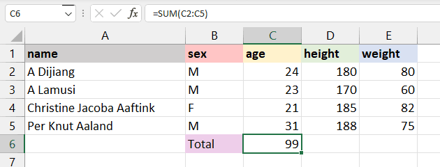

Check out our full guide on how to sum in Excel to learn more.

2. MIN() and MAX()

The MIN() function requires a range of cells, and it returns the minimum value. For example, we want to display the minimum weight among all athletes on the E6 cell. The MIN() function will search for the minimum value and show 60.

=MIN(E2:E5)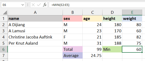

The MAX() function is the opposite of MIN(). It will return the maximum value from the selected range of cells. The function will look for the maximum value and return 82. 

=MAX(E2:E5)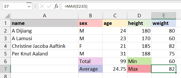

3. AVERAGE()

The AVERAGE() function calculates the average of selected cells. You can provide a range of cells (C2:C5) or select individual cells (C2, C3, C5).

To calculate the average of athletes, we will select the age column, apply the average function, and return the result to the C7 cell. It will sum up the total values in the selected cells and divide them by 4.

=AVERAGE(C2:C5)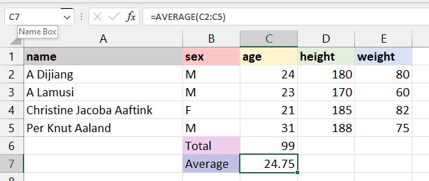 

We have a separate, detailed guide on AVERAGE() in Excel if you want to learn more.

4. COUNT()

The COUNT() function counts the total number of selected cells. It will not count the blank cells and different data formats other than numeric. 

We will count the total number of athlete weights, and it will return 4, as we don’t have missing values or strings. 

=COUNT(E2:E5)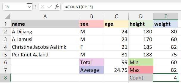

To count all types of cells (date-time, string, numerical), you need to use the COUNTA() function. 

The COUNTA() function does not count missing values. For blank cells, use COUNTBLANK().

If you want some more examples of how to use COUNT() in Excel, check out our separate guide. 

5. POWER()

In the beginning, we learned to add power using ^, which is an alternative to the POWER() function. Use either x^y or POWER(x,y); POWER can be clearer in nested formulas to square, cube, or apply any raise to power to your cell.

In our case, we have divided D2 by 100 to get height in meters and squared it by using the POWER() function with the second argument as 2.   

=POWER(D2/100,2)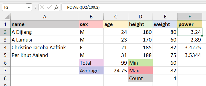

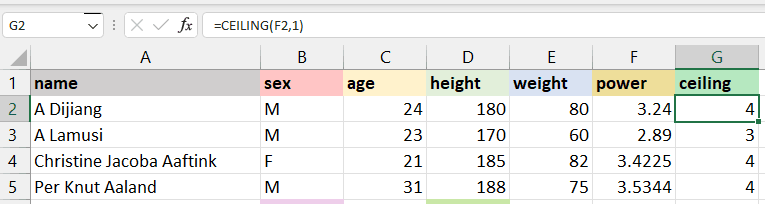
6. CEILING() and FLOOR()

As we explore in our guide on Excel ROUND(), the CEILING() function in Excel rounds a number up to the nearest specified multiple. For example:

• =CEILING(3.24, 1) rounds 3.24 up to 4.
• =CEILING(3.24, 5) rounds 3.24 up to 5.

Let's look at a worked example below. You'll see that we round F2 to a multiple of 1 and get 4. 

=CEILING(F2,1)

Optional: =CEILING.MATH(F2,1)

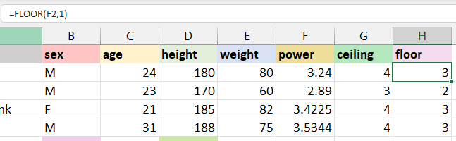
In contrast, the FLOOR() function rounds a number down to the nearest specified multiple. For instance:

• =FLOOR(3.24, 1) rounds 3.24 down to 3.
• =FLOOR(3.24, 5) rounds 3.24 down to 0.

As we can see in the example below, instead of converting 3.24 to 4, it has rounded the number to 3. 

=FLOOR(F2,1)

Optional: =FLOOR.MATH(F2,1)

These functions are especially useful when working with standardized intervals, such as rounding prices, time, or quantities to fixed units.

7. CONCAT()

The CONCAT() Excel function joins strings. Prefer CONCAT or TEXTJOIN over legacy CONCATENATE; use TEXTJOIN when you need a delimiter or to ignore blanks. For example, if we want to join the age and sex of the athletes, we will use CONCAT(). The function will automatically convert a numeric value from age to string and combine it. 

“24”+“M” = “24M”

=CONCAT(C2,B2)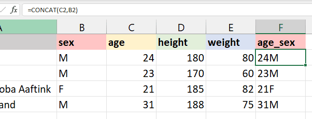

Find out more about this function and how it's used in our guide on how to use Excel CONCAT().

8. TRIM()

As we learned in our full guide on TRIM() in Excel, this function is used to remove extra spaces from the start, middle, and end. It is commonly used to identify duplicate values in cells, and for some reason, extra space makes it unique.  

For example:

1. There are extra two spaces at A3 “A   Lamusi”, and it has been successfully removed by TRIM().
2. At A4 “ Christie Jacoba Aaftink”, there is extra space at the start, and without writing any complex function, TRIM() has removed it. 

=TRIM(A4)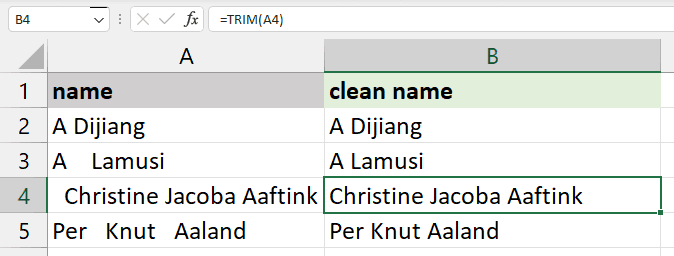

9. REPLACE() and SUBSTITUTE()

REPLACE() is used for replacing part of the string with a new string.

REPLACE(old_text, start_num, num_chars, new_text) 

• old_text is the original text or cell containing the text.

• start_num is the index position that you want to start replacing the character. 

• num_chars refers to the number of characters you want to replace.

• new_text indicates the new text that you want to replace with old text.

For example, we will change A Dijiang with B Dijiang by providing the positing of character, which is 1, the number of characters that we want to replace, which is also 1, and the new character “B”. 

=REPLACE(A2,1,1,"B")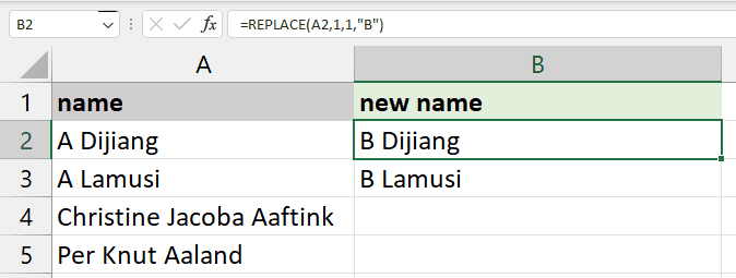

The SUBSTITUTE() function is similar to REPLACE(). Instead of providing the location of a character or the number of characters, we will only provide old text and new text. 

SUBSTITUTE(text, old_text, new_text, [instance_num])

Note:  Use instance_num to replace only a specific occurrence

In our case, we are replacing "Jacoba" with "Rahim" to display the result on A4 cell “Christine Rahim Aaftink.”

This function is quite useful as it does not change the text without “Jacoba” as shown below in cell A5, “Per Knut Aaland.” Whereas, REPLACE() will replace the text every time. 

=SUBSTITUTE(A4,"Jacoba","Rahim")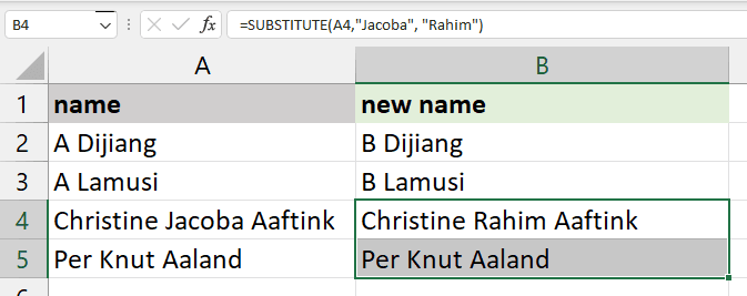

10. LEFT(), RIGHT(), and MID()

The LEFT() function returns the number of characters from the start of the string or text. 

For example, to display the first name from the text “Christine Jacoba Aaftink”, you will use LEFT() with 9 numbers of characters. As a result, it will show the first nine characters; “Christine.”

=LEFT(A2,9)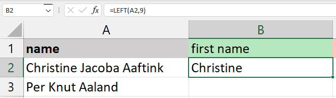

The MID() function requires a starting position and length to extract the characters from the middle. 

For example, if you want to display a middle name, you will start with “J” which is at the 11th position, and 6 for the length of the middle name “Jacoba”.

=MID(A2,11,6)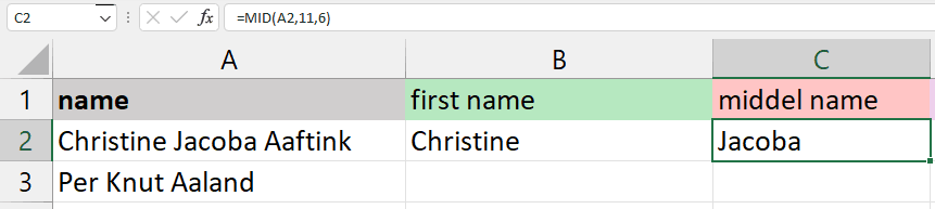

The RIGHT() function will return the number of characters from the end. You just need to provide a number of characters. 

For example, to display the last name “Aaftink,” we will use RIGHT() with seven characters. 

=RIGHT(A2,7)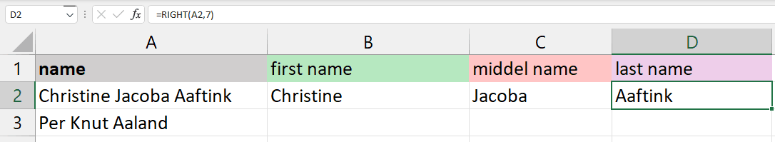

11. UPPER(), LOWER(), and PROPER()

The UPPER(), LOWER(), and PROPER() functions are basic string operations. You can find similar in Tableau or in Python. These functinos only require a text, the location of the cell containing string, or the range of cells with string. 

UPPER() will convert all the letters in the text to uppercase. 

=UPPER(A1)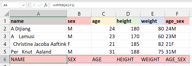

LOWER() will convert the selected text to lowercase.

=LOWER(A1)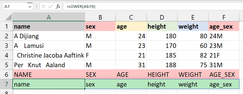

PROPER() will convert the string to the proper case. For example, the first letter in each word will be capitalized, and the rest of them will be lowercase. 

=PROPER(A1)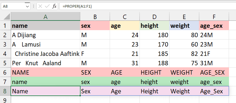

12. NOW() and TODAY()

NOW() returns the current time and date, and TODAY() returns only the current date. These are quite simple, and we will use them to extract a day, month, year, hours, and minutes from any date time data cell. 

The example below returns the current date and time.

=NOW()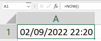

To extract the seconds from the time, you will use the SECOND() function. 

=SECOND(NOW())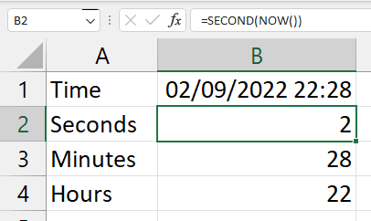

Similarly, TODAY() will return only the current date. 

=TODAY()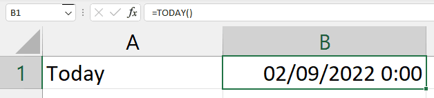

To extract the day, you will use the DAY() function.

Furthermore, you can extract month, year, weekday, day names, hours, and minutes from the date time data field. 

=DAY(TODAY())

13. DATEDIF()

It is the most used function for time series data sets. The DATEDIF() calculates the difference between two dates and returns the number of days, months, weeks, or years based on your preference. 

Caution: DATEDIF is a legacy compatibility function and can be inaccurate in some units (e.g., "MD"). Consider DAYS(), YEARFRAC(), or DATE arithmetic when possible.

In the example below, we want to return the date difference in days by providing “d” for unit arguments. Make sure that the first argument is the start date and the second argument in the function is the end date. 

start_date < end_date

=DATEDIF(A2,B2,"d")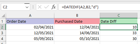

14. VLOOKUP() and HLOOKUP()

The worksheet1 that we will use in this section contains all the data from the Olympics dataset.

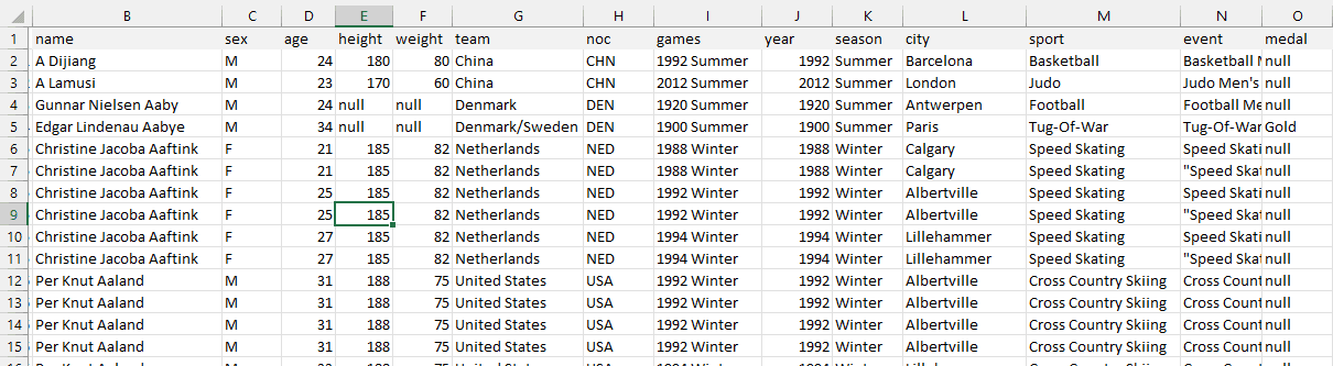
worksheet1

The VLOOKUP() function searches for the value in the leftmost column of the table array and returns the value from the same row from the specified columns. 

Note: VLOOKUP() and HLOOKUP() are legacy/compatibility functions. Microsoft recommends using XLOOKUP() for new work because it replaces both, returns exact matches by default, can search in any direction, and has an if_not_found argument. You can read our guide on how to use XLOOKUP to learn more, and check out a comparison of XLOOKUP vs VLOOKUP to see the difference.

VLOOKUP(lookup_value, table_array, col_index, range_lookup)

• lookup_value: the value you are looking for that is present in the first column. 

• table_array: the range of the table, worksheet, or selected cell with multiple columns. 

• col_index: the position of the column to extract the value.

• range_lookup: “True” is used for the approximate match (default), and “FALSE” is used for the exact match.

In our case, we are looking for A Dijiang (A2) from selected columns and rows of worksheet1 (B2:H20). The VLOOKUP() function will check the name column in worksheet one and return the 6th column value that is team “China”.

=VLOOKUP(A2,worksheet1!B2:H20,6,FALSE)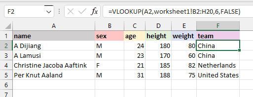

HLOOKUP() searches for the value in the first row instead of the first column. It returns the value from the same column and the row you specified. 

HLOOKUP(lookup_value, table_array, row_index, range_lookup)

In our case, we will display A Dijaing’s sex on the D8 cell. The HLOOKUP() function will look for the name in the first row and return the value “M'' from the 2nd row of the same column. The range_lookup is kept FALSE in both cases for the exact match. 

=HLOOKUP(B1,B1,E5,2,FALSE)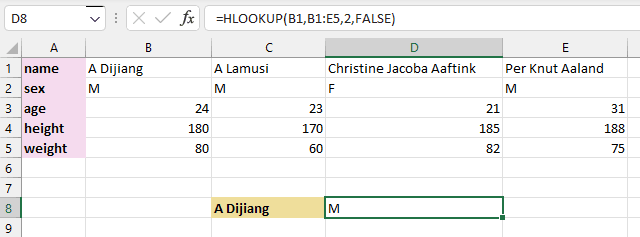

15. IF()

The IF() Excel function is straightforward. It is similar to an if-else statement in a programming language. We will provide the logic of the function. If the logic is correct, it will return a certain value; if the logic is false, it will return a different value. 

For example, if the BMI of an athlete is less than 24.9, the function will return the string “Fit”, else “Unfit”. It is quite useful to convert numerical values into categories. 

=IF(G2<24.9,"Fit","Unfit")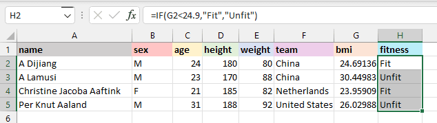

Other Kinds of Formulas in Excel

Now, let's look at other kinds of Excel formulas, including formulas using operators, array formulas, and formula-based conditional formatting.

Formulas using operators

Even something as simple as A1 + A2 is a formula because it performs a calculation using cell references and an operator, just like more complex formulas. Excel can also update the result dynamically based on changes in A1 or A2. All of these count as formulas:

• Addition: =A1 + B1

• Subtraction: =A1 - B1

• Multiplication: =A1 * B1

• Division: =A1 / B1

All this seems basic but it is also the foundation of more advanced patterns like sequences and recursive calculations. Here is how we might create a Fibonacci sequence:

• Enable iterative calculations by going to File > Options > Formulas and clicking Enable Iterative Calculation. Set the maximum iterations. 
• Enter the following in cell A3 (assuming A1=0 and A2=1) and drag down. 

Array formulas

Array formulas perform multiple calculations at once and return either a single result or multiple values across a range of cells. They are particularly useful for operations that involve multiple conditions or when you are doing calculations in large datasets.

Here is an example where we are doing the sum of squared values in a range: =SUM(A1:A5^2). This might be useful if you are thinking about something like regression in Excel. You can see that this is a formula because it begins with the equal sign and performs a calculation, but it's also more than just the earlier SUM() function example because of the caret.  

Formula-based conditional formatting

Excel allows users to apply conditional formatting using custom formulas rather than predefined rules. For example, a formula that applies formatting based on row-specific conditions across multiple columns wouldn't work as a regular cell formula but works correctly within conditional formatting. 

Here is an example where we highlight an entire row if a cell meets a condition. For this example, we imagine a table where column C contains order statuses ("Pending" or "Shipped"), and we want to highlight entire rows where the status is "Pending." Here are the steps.

1. Select the entire range of your table (e.g., A2:E100).
2. Go to Home > Conditional Formatting > New Rule.
3. Select Use a formula to determine which cells to format.
4. Enter this formula: =$C2="Pending"
5. Click Format, choose a fill color, and press OK.

This formula looks similar to something you can put in a single cell of your workbook. However, this formula is applied relative to each row but works across the entire selected range. So, in a cell, =$C2="Pending" would just return TRUE or FALSE, but in conditional formatting, Excel applies formatting to entire rows dynamically based on our logic.

Upskilling Your Team in Excel

We've covered the Excel formulas that everyone needs to know, but upskilling multiple people in this area isn't always straightforward. We have a separate guide that covers corporate Excel training in depth, but it's worth mentioning here.

We've established that Excel is more than just a spreadsheet tool—it's often essential for effective data management, financial analysis, and decision-making. As such, investing in Excel training can boost your team's productivity, accuracy, and overall efficiency. Key benefits include:

• Data analysis: Advanced Excel skills enable more insightful data interpretation, aiding better decision-making.
• Efficiency: Automation through spreadsheets can reduce manual work and errors.
• Financial precision: Mastery of functions like VLOOKUP and pivot tables enhances financial management.
• Operational streamlining: Excel's data manipulation tools can improve the handling of large datasets, optimizing operations.
• Competitive edge: Proficiency in Excel provides a significant advantage in refining processes and gaining insights.

If you're looking to train your team in Excel skills, from the basics to more advanced formulas, DataCamp For Business is the ideal tool. Whether your team is 2 people or 10,000 people, DataCamp For Business offers a host of dedicated Excel and spreadsheet learning materials, the ability to create custom tracks to scale and tailor your learning experience, and detailed reporting and insights to measure the impact of your training. Request a demo today to get started. 

Conclusion

Microsoft Excel is a powerful and easy-to-use application for data analysis and reporting. In this post, we have learned the importance of basic Excel formulas and how they provide us extra ability to perform complex calculations. Furthermore, we have learned about various ways of adding formulas to worksheets and looked in detail at the essential basic Excel formulas. 

To learn more about Excel and how to use these formulas for data analysis, take our Data Analysis in Excel course. It will teach you the basics of data exploration, processing, and analysis. If you are fond of the Google stack and use Google Sheets, try Data Analysis in Spreadsheet.

You can also take another step forward by learning the fundamentals of a spreadsheet. You will learn about data analysis, advanced data manipulation techniques, pivot tables, and data visualization. Finally, you can check out our Excel Formulas cheat sheet for a quick reference guide and learn more about data types in Excel.