Python Dictionary Methods: A Complete Guide

For any data scientist or software engineer, the ability to efficiently map relationships between data points is a non-negotiable skill. If you are parsing complex JSON responses from an API, aggregating statistics from a massive dataset, or simply configuring application settings, then a dictionary is arguably Python's most powerful tool. It drives clean, readable, and highly optimized data manipulation.

While anyone can look up a value in a dictionary, real expertise shows when you know how to apply its methods to your data workflows and unlock advanced patterns.

In this article, we’ll look at hash tables that make dictionaries so fast, essential dictionary methods, error handling strategies, and performance optimization techniques. 

If you're new to dictionaries, I recommend reading our foundational Python Dictionary tutorial as a good starting point.

What Are Python Dictionaries?

Python dictionaries are a built-in data structure designed for fast, flexible lookups. They allow you to store and retrieve values using meaningful keys rather than numeric positions, which makes them ideal for representing structured, real-world data. Let’s look at their core structure and properties.

Core dictionary architecture and hashing

Before we get into the details of Python’s dictionary methods, it helps to understand how dictionaries are built on hash tables. Many of the errors you’ll run into, like TypeError: unhashable type, come straight from the way this structure works.

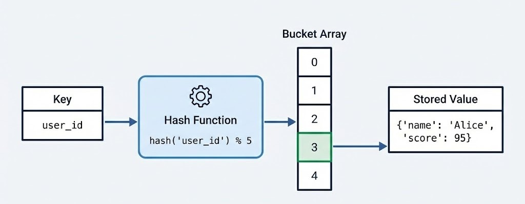
At a structural level, a Python dictionary implements a hash table. This architectural choice is what gives the dictionary its speed and versatility. When you define a dictionary, you are essentially creating a sparse array, often called a bucket array.

When you insert a key-value pair, Python passes the key through a hash function. This function calculates a unique integer (the hash) that determines the specific index in the bucket array where the value will be stored.

Because of this design:

• Keys must be hashable, which usually means they must be of an immutable type (e.g., str, int, tuple)

• Values can be mutable, including lists, other dictionaries, or custom objects

• Lookups, insertions, and deletions run in average amortized O(1) time

The following example shows a few valid keys, but also demonstrates that a list is not accepted as dictionary key:

# Valid dictionary - immutable keys, any values
user_data = {
    "name": "Alice",           # string key, string value
    42: [1, 2, 3],             # integer key, list value
    (10, 20): {"nested": True} # tuple key, dict value
}
print(type(user_data), "valid dict")

# Invalid - will raise TypeError
try:
    invalid_dict = {[1, 2]: "value"}  # lists are not hashable
except TypeError as e:
    print(f"Error: {e}")

<class 'dict'> valid dict
Error: unhashable type: 'list'

This structure is important for performance. While searching for an item in a list requires iterating through elements one by one, an O(n) operation, retrieving a value from a dictionary is an O(1) operation on average. 

This means looking up a user ID in a dataset of one million users takes roughly the same amount of time as looking it up in a dataset of ten users. Understanding the differences between data types in Python is key to choosing the right structure for your use case.

Evolution of order and properties

One of the most significant changes in Python's history occurred in version 3.7. Before this, dictionaries were considered unordered collections, and iterating over them could produce keys in seemingly random sequences. If you printed a dictionary, the items might appear in a different order than you inserted them, depending on the hash values and the internal array history.

However, starting with Python 3.6, dictionaries began preserving insertion order as an implementation detail in CPython. Then, beginning with Python 3.7 (and officially guaranteed in the language specification), dictionaries preserve insertion order. 

This shift from unordered to ordered mappings has a few important implications for modern Python development. For instance, JSON serialization now produces predictable output, which makes debugging easier and ensures data reproducibility across different runs. 

If you're working with data pipelines where order matters, such as processing time-series events or maintaining configuration hierarchies, this guarantee eliminates an entire class of subtle bugs. Next, let’s see how to create a dictionary.

Creating a Python Dictionary

While creating a dictionary seems straightforward, the method you choose can impact both the readability and performance of your code. Python provides multiple ways for initialization, which range from simple literals to advanced programmatic generation techniques for data science workflows. Let’s look at the most important ways.

Curly brace literals

The most common and preferred way to create a dictionary is using curly brace syntax {}. This literal notation is not only more readable but also faster than alternative methods. Python can optimize the bytecode construction directly without the overhead of a function call. Below is the code showing a dictionary:

# Preferred: Literal syntax
user_profile = {
    "name": "Alice",
    "role": "Data Scientist",
    "active": True
}
user_profile

{'name': 'Alice', 'role': 'Data Scientist', 'active': True}

dict() constructor

However, the dict() constructor is indispensable in a few scenarios. It acts as a type converter, allowing you to build dictionaries from sequences of tuples or keyword arguments. It is particularly useful in these specific cases: 

• Keys are valid Python identifiers, but you want to avoid quoting strings 
• You need to transforming data structures like lists of paired values

# Using keyword arguments (cleaner for string keys)
config = dict(host="localhost", port=8080, debug=True)
print(config)

# Converting a list of tuples (common in data processing)
pairs = [("a", 1), ("b", 2), ("c", 3)]
lookup_table = dict(pairs)
print(lookup_table)

{'host': 'localhost', 'port': 8080, 'debug': True}
{'a': 1, 'b': 2, 'c': 3}

Dictionary comprehensions

For more complex dictionary creation scenarios, dictionary comprehensions offer a concise and efficient way to filter, transform, or generate key-value pairs programmatically. It’s an essential technique for any data practitioner who needs to process and reshape data dynamically.

Comprehensions are vital for tasks like:

• Inverting a dictionary
• Filtering out null values from a dataset

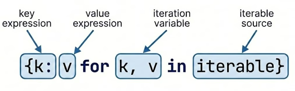
Let’s see how to create a dictionary comprehension below:

# Classic use case: Creating a squares map
squares = {x: x**2 for x in range(5)}
print(squares)

# Filtering data during creation
raw_data = {"a": 10, "b": None, "c": 5}
clean_data = {k: v for k, v in raw_data.items() if v is not None}
print(clean_data)

{0: 0, 1: 1, 2: 4, 3: 9, 4: 16}
{'a': 10, 'c': 5}

If you want to dive deeper, I recommend you go through our Python Dictionary Comprehension tutorial.

dict.fromkeys()

Another useful Python dictionary method for initialization is dict.fromkeys(). This method creates a new dictionary with specified keys and a single value. It is often used to initialize counters or status flags.

# Initialize multiple keys with the same default value
categories = ["electronics", "clothing", "food", "books"]
inventory = dict.fromkeys(categories, 0)
print(inventory) 

# Initialize with None for optional fields
user_fields = ["email", "phone", "address", "company"]
user_profile = dict.fromkeys(user_fields)
print(user_profile)

{'electronics': 0, 'clothing': 0, 'food': 0, 'books': 0}
{'email': None, 'phone': None, 'address': None, 'company': None}

When using .fromkeys() with mutable objects like lists or dictionaries, all keys will reference the same object in memory. This creates a “shared reference” pitfall that can lead to unexpected behavior. Let’s see this with an example:

# DANGEROUS - all keys share the same list!
categories = ["A", "B", "C"]
wrong_way = dict.fromkeys(categories, [])
wrong_way["A"].append(1)
print(wrong_way) 

# CORRECT - use dictionary comprehension for independent lists
right_way = {cat: [] for cat in categories}
right_way["A"].append(1)
print(right_way)

{'A': [1], 'B': [1], 'C': [1]}
{'A': [1], 'B': [], 'C': []}

We can see that the same value was shared by all keys in the first case. To avoid this, we need to use a dictionary comprehension for independent lists.

Python Dictionary Methods For Access and Modification

Once a dictionary is created, interacting with the data stored inside is one of the most common daily programming tasks. Let’s look at some of these ways.

Accessing and retrieving values

There are a few different ways to access values.

Bracket notation

The most direct way to retrieve a value from a dictionary is through bracket notation d[key], which returns the associated value if the key exists. This approach is ideal when you're confident the key is present in your dictionary. Below is the code to do it:

product = {
    "name": "Laptop",
    "price": 1299.99,
    "stock": 45,
    "category": "Electronics"
}

# Direct access with brackets
print(product["name"]) 
print(product["price"]) 

# Attempting to access a non-existent key raises KeyError
try:
    print(product["manufacturer"])
except KeyError as e:
    print(f"Key not found: {e}")

Laptop
1299.99
Key not found: 'manufacturer'

.get() method

For safer retrieval when key existence is uncertain, the .get() method provides an elegant solution. It returns None (or a specified default value) instead of raising an exception if the key doesn't exist.

# Safe retrieval with .get()
manufacturer = product.get("manufacturer")
print(manufacturer)  # None

# Provide a custom default value
warranty = product.get("warranty", "No warranty information")
print(warranty)

# .get() is especially useful in data pipelines
customer_data = {"name": "John Doe", "email": "john@example.com"}

phone = customer_data.get("phone", "Not provided")
print(phone)

address = customer_data.get("address", "Not provided")
print(address)

None
No warranty information
Not provided
Not provided

.setdefault() method

The .setdefault() method combines retrieval and insertion in a single operation. It retrieves a value if the key exists, or inserts a default value and returns it if the key is missing, which is perfect for accumulation patterns.

# Using .setdefault() for initialization and retrieval
page_visits = {}

# First visit to 'home' - inserts 0 and returns it
count = page_visits.setdefault("home", 0)
print(count) 
page_visits["home"] += 1

# Subsequent call returns existing value
count = page_visits.setdefault("home", 0)
print(count)

# Practical example: grouping items
inventory = [
    ("apple", "fruit"),
    ("carrot", "vegetable"),
    ("banana", "fruit"),
    ("broccoli", "vegetable")
]

grouped = {}
for item, category in inventory:
    grouped.setdefault(category, []).append(item)

print(grouped)

0
1
{'fruit': ['apple', 'banana'], 'vegetable': ['carrot', 'broccoli']}

Modifying dictionaries

Dictionaries are dynamic; you will often need to add or remove data as your program executes. 

Adding key-value pairs with the .update() method

Adding a single pair is as simple as assignment (d['new'] = 1), but for bulk operations, the .update() method is superior. It accepts another dictionary or an iterable of key-value pairs, and merges them into the existing object.

Let’s see how to use the .update() method:

# Simple assignment for single key-value pairs
user = {"username": "alice_2024", "role": "analyst"}
user["email"] = "alice@company.com"  # Add new key
user["role"] = "senior_analyst"      # Update existing key

# Bulk update with .update()
user.update({"department": "Analytics", "level": 3})
print(user)

# Update from sequence of tuples
additional_info = [("projects", 12), ("rating", 4.8)]
user.update(additional_info)
print(user)

# Update with keyword arguments
user.update(active=True, certified=True)
print(user)

{'username': 'alice_2024', 'role': 'senior_analyst', 'email': 'alice@company.com', 'department': 'Analytics', 'level': 3}
{'username': 'alice_2024', 'role': 'senior_analyst', 'email': 'alice@company.com', 'department': 'Analytics', 'level': 3, 'projects': 12, 'rating': 4.8}
{'username': 'alice_2024', 'role': 'senior_analyst', 'email': 'alice@company.com', 'department': 'Analytics', 'level': 3, 'projects': 12, 'rating': 4.8, 'active': True, 'certified': True}

For a detailed walkthrough on adding items, I recommend you go through this guide on Python Dictionary Append.

Removing items from a dictionary

Python offers three distinct methods for removing dictionary entries, each with different behavior and use cases:

• .pop(key): Removes the key and returns its value. This is useful when you need to use the data one last time before deleting it.

• .popitem(): Removes and returns the last inserted key-value pair (LIFO). This is a direct benefit of the ordered nature of modern dictionaries.

• del d[key]: purely deletes the key. It does not return the value and is slightly faster if the return value is not needed.

Let’s see examples of these methods:

.pop() method:

scores = {"Alice": 95, "Bob": 87, "Carol": 92, "David": 78}

# .pop() - removes key and returns its value
alice_score = scores.pop("Alice")
print(alice_score)
print(scores) 

95
{'Bob': 87, 'Carol': 92, 'David': 78}

.popitem() method:

# .popitem() - removes and returns last inserted pair (LIFO in Python 3.7+)
scores = {"Alice": 95, "Bob": 87, "Carol": 92, "David": 78}
last_item = scores.popitem()
print(last_item)
print(scores)

('David', 78)
{'Alice': 95, 'Bob': 87, 'Carol': 92}

del:

# del statement - removes key without returning value
scores = {"Alice": 95, "Bob": 87, "Carol": 92, "David": 78}
del scores["Bob"]
print(scores)

{'Alice': 95, 'Carol': 92, 'David': 78}

Emptying a dictionary with the .clear() method

The .clear() method empties the entire dictionary, leaving you with an empty {} object. This is distinct from deleting the variable itself. The object remains in memory, just empty. Let’s see how this method works:

# .clear() - removes all items but keeps the dictionary object
scores = {"Alice": 95, "Bob": 87, "Carol": 92, "David": 78}
scores.clear()
print(scores)
print(type(scores))

{}
<class 'dict'>

The distinction between these methods matters. Use .pop() when you need the removed value, .popitem() for stack-like behavior, del for simple removal, and .clear() to reset a dictionary while preserving its identity.

Views and iteration

In older versions of Python 2, methods like .keys() returned a static list. In the current versions of Python (3.x), these return view objects. Views are dynamic windows into the dictionary. If the dictionary changes, the view reflects those changes instantly without needing to be re-called.

Iterating through .keys(), .values(), and .items()

You can iterate through keys (.keys()), values (.values()), or both simultaneously using .items(). Let’s see these methods with an example:

experiment = {
    "model": "RandomForest",
    "accuracy": 0.94,
    "precision": 0.91,
    "recall": 0.89
}

# .keys() returns a view of all keys
print(experiment.keys()) 

# .values() returns a view of all values
print(experiment.values())

# .items() returns (key, value) tuples - most commonly used
for metric, value in experiment.items():
    if isinstance(value, float):
        print(f"{metric}: {value:.2%}")

dict_keys(['model', 'accuracy', 'precision', 'recall'])
dict_values(['RandomForest', 0.94, 0.91, 0.89])
accuracy: 94.00%
precision: 91.00%
recall: 89.00%

The dynamic nature of view objects means they automatically reflect changes made to the dictionary after the view is created. Let’s see an example:

metrics = {"MAE": 0.23, "RMSE": 0.45}
keys_view = metrics.keys()
print(keys_view)

# Add new metric
metrics["R2"] = 0.87
print(keys_view)

dict_keys(['MAE', 'RMSE'])
dict_keys(['MAE', 'RMSE', 'R2'])

Intersections and unions

A powerful feature of view objects is that they support set operations. You can perform them directly on key views to compare two dictionaries efficiently using these operators:

• Intersection: &

• Union: |

• Difference: -

• Symmetric difference/XOR: ^

Let’s see an example:

dict1 = {"a": 1, "b": 2, "c": 3}
dict2 = {"b": 20, "c": 30, "d": 4}

# Find common keys (intersection)
common_keys = dict1.keys() & dict2.keys()
print(common_keys)

# Find all unique keys (union)
all_keys = dict1.keys() | dict2.keys()
print(all_keys)

# Find keys in dict1 but not in dict2 (difference)
unique_to_dict1 = dict1.keys() - dict2.keys()
print(unique_to_dict1)

# Symmetric difference - keys in either but not both
exclusive_keys = dict1.keys() ^ dict2.keys()
print(exclusive_keys)

{'b', 'c'}
{'b', 'c', 'd', 'a'}
{'a'}
{'d', 'a'}

These view-based set operations are far more memory-efficient than converting dictionaries to sets explicitly, especially when working with large datasets.

Avoiding Errors In Python Dictionary Methods

Because dictionaries are often used as the primary interface for external data, such as JSON payloads from APIs or configuration files, they are a common source of runtime errors. Writing robust code requires more than just knowing how to access data. It requires knowing how to handle its absence. 

The most common dictionary error is KeyError, which occurs when attempting to access a key that doesn't exist. Python offers two philosophical approaches to handling this: 

• EAFP (Easier to Ask Forgiveness than Permission) 
• LBYL (Look Before You Leap)

EAFP: Managing KeyError and exceptions

The EAFP pattern is considered more Pythonic and often performs better when keys usually exist, as it avoids redundant checks.  It uses try-except blocks to handle errors after they occur, assuming that operations will usually succeed. Let’s see how this works:

# EAFP approach - try first, handle exceptions
user_data = {"username": "data_analyst", "email": "analyst@company.com"}

try:
    phone = user_data["phone"]
    print(f"Phone: {phone}")
except KeyError:
    print("Phone number not available")
    phone = None

# More sophisticated error handling with specific actions
config = {"host": "localhost", "port": 5432}

try:
    database = config["database"]
except KeyError:
    print("Warning: Database not specified, using default")
    database = "default_db"
    config["database"] = database  # Add missing configuration

Phone number not available
Warning: Database not specified, using default

However, there are scenarios where failing loudly, allowing the KeyError to propagate, is actually preferable to silent failures. In the LBYL approach, you explicitly check for the key's existence before accessing it. Let’s see an example:

# Critical configuration - fail loudly if missing
required_config = {"api_key": "secret123", "endpoint": "api.example.com"}

def initialize_api(config):
    # Don't catch KeyError - we WANT the program to crash if required keys are missing
    api_key = config["api_key"]
    endpoint = config["endpoint"]
    timeout = config.get("timeout", 30)  # Optional with default
    
    return {"key": api_key, "endpoint": endpoint, "timeout": timeout}

Invoking this function with will raise KeyError if any key in the dictionary is missing, which is correct behavior because it is better to fail during initialization than silently during production.

Explicit error handling

When processing data from external sources like APIs or user input, explicit error handling becomes important. Let’s see how to do it with an example:

# Processing API response with defensive error handling
def extract_user_info(api_response):
    """Extract user information with comprehensive error handling."""
    user_info = {}
    
    try:
        user_info["id"] = api_response["user"]["id"]
        user_info["name"] = api_response["user"]["profile"]["name"]
    except KeyError as e:
        print(f"Missing required field in API response: {e}")
        return None
    
    # Optional fields - use .get() with defaults
    user_info["email"] = api_response.get("user", {}).get("contact", {}).get("email", "N/A")
    user_info["verified"] = api_response.get("user", {}).get("verified", False)
    
    return user_info

# Example usage
response = {
    "user": {
        "id": 12345,
        "profile": {"name": "Jane Smith"},
        "verified": True
    }
}

user = extract_user_info(response)
print(user)

{'id': 12345, 'name': 'Jane Smith', 'email': 'N/A', 'verified': True}

Understanding when to use .get() versus bracket notation versus try-except is important. 

LBYL: Proactive membership testing

The LBYL approach uses conditional statements using the  in and not in operators to check for key existence before attempting access. This pattern is clearer when dealing with conditional logic or when you need to take different actions based on key presence. Let’s see an example of this:

# Proactive checking with 'in' operator
student_grades = {
    "Alice": 95,
    "Bob": 87,
    "Carol": 92
}

# Check before access
student_name = "David"
if student_name in student_grades:
    print(f"{student_name}'s grade: {student_grades[student_name]}")
else:
    print(f"No grade recorded for {student_name}")

# Conditional update based on existence
if "David" not in student_grades:
    student_grades["David"] = 0  # Initialize new student
    print("New student added to grading system")

# Multiple key checks for validation
required_fields = ["name", "email", "department"]
employee_record = {"name": "John Doe", "email": "john@company.com"}

missing_fields = [field for field in required_fields if field not in employee_record]
if missing_fields:
    print(f"Error: Missing required fields: {missing_fields}")
else:
    print("All required fields present")

No grade recorded for David
New student added to grading system
Error: Missing required fields: ['department']

When validating dictionaries derived from external sources such as JSON from APIs, CSV files, or user input, proactive membership testing provides clear, readable validation logic. Let’s see this with an example:

# Validating API response structure
def validate_product_data(product):
    """Validate product dictionary has all required fields."""
    required = ["id", "name", "price", "category"]
    optional = ["description", "stock", "manufacturer"]
    
    # Check all required fields exist
    for field in required:
        if field not in product:
            raise ValueError(f"Missing required field: {field}")
    
    # Validate data types for existing fields
    if "price" in product and not isinstance(product["price"], (int, float)):
        raise TypeError("Price must be a number")
    
    if "stock" in product and product["stock"] < 0:
        raise ValueError("Stock cannot be negative")
    
    return True

# Example usage with proper error handling
product_from_api = {
    "id": 101,
    "name": "Wireless Mouse",
    "price": 29.99,
    "category": "Electronics",
    "stock": 150
}

try:
    if validate_product_data(product_from_api):
        print("Product data validated successfully")
        # Proceed with processing
except (ValueError, TypeError) as e:
    print(f"Validation failed: {e}")

Product data validated successfully

Choosing the right approach

The choice between EAFP and LBYL often depends on your use case. Use EAFP when operations typically succeed and exceptions are rare. Use LBYL when you need explicit branching logic or when validating input before expensive operations.

Before iterating over a dictionary derived from an external source, it is best practice to:

• Validate early
• Check all required keys at once
• Raise specific and informative exceptions
• Clearly separate required fields from optional ones
• Validate more than just presence when needed
• Prefer explicit failure over silent fallbacks

By following these practices, you can make your code much more robust when dealing with unpredictable or incomplete data from APIs, user input, or configuration files.

For a more deeper look into writing resilient Python code, I recommend taking our course on Writing Efficient Python Code.

Advanced Python Dictionary Methods

As your data science projects grow in complexity, you’ll often need to combine, copy, and transform dictionaries. Learning these advanced operations enables you to manipulate data structures efficiently while avoiding subtle bugs that can derail pipelines. Let’s see some of these methods.

Merging operators

Python 3.9 introduced elegant union operators for merging dictionaries:

• | (merge operator): Creates a new merged dictionary.

• |= (update operator): Updates an existing dictionary in place.

These operators provide clean, readable syntax for combining data from multiple sources. Let’s see an example:

# Union operator | creates a new merged dictionary
defaults = {"theme": "light", "language": "en", "notifications": True}
user_prefs = {"theme": "dark", "font_size": 14}

final_config = defaults | user_prefs
print(final_config)

# Update operator |= modifies in place
settings = {"auto_save": True, "theme": "light"}
settings |= {"theme": "dark", "font_size": 12}
print(settings)

{'theme': 'dark', 'language': 'en', 'notifications': True, 'font_size': 14}
{'auto_save': True, 'theme': 'dark', 'font_size': 12}

For Python versions before 3.9, the double-star unpacking method (**) provides similar functionality:

# Double-star unpacking
base_config = {"host": "localhost", "port": 5432, "ssl": False}
override_config = {"port": 5433, "ssl": True, "timeout": 30}

# Merge using unpacking
merged = {**base_config, **override_config}
print(merged)

# Multiple dictionary merge
db_config = {"database": "analytics"}
auth_config = {"username": "admin", "password": "secret"}
pool_config = {"pool_size": 10, "max_overflow": 20}

complete_config = {**db_config, **auth_config, **pool_config}
print(complete_config)

{'host': 'localhost', 'port': 5433, 'ssl': True, 'timeout': 30}
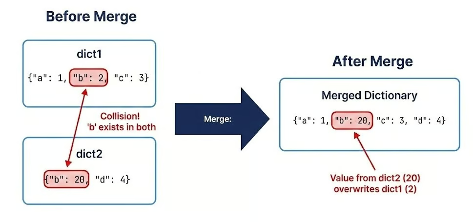
{'database': 'analytics', 'username': 'admin', 'password': 'secret', 'pool_size': 10, 'max_overflow': 20}

Collision precedence

Across all merging techniques, the rule is simple: last seen wins. The value from the right-hand dictionary overwrites the left-hand one if keys collide:

dict1 = {"a": 1, "b": 2, "c": 3}
dict2 = {"b": 20, "c": 30, "d": 4}
dict3 = {"c": 300, "e": 5}

result = dict1 | dict2 | dict3
print(result)

result2 = {**dict1, **dict2, **dict3}
print(result2)

# Order matters - reversing changes the result
result3 = dict3 | dict2 | dict1
print(result3)

{'a': 1, 'b': 20, 'c': 300, 'd': 4, 'e': 5}
{'a': 1, 'b': 20, 'c': 300, 'd': 4, 'e': 5}
{'c': 3, 'e': 5, 'b': 2, 'd': 4, 'a': 1}

This behavior is consistent whether you use |, |=, unpacking, or the .update() method. Order matters, making it especially useful for layered configuration management (e.g., system defaults < environment configs < user overrides).

Copying mechanisms

One of the most dangerous pitfalls is misunderstanding how Python handles variable assignments. 

Reference assignments create aliases, not copies

dict_a = dict_b does not create a copy. It creates a reference (an alias). Modifying one modifies the other. The following example illustrates the concept:

# Reference assignment - creates an alias, not a copy
original = {"name": "Dataset_v1", "records": 1000}
alias = original

# Modifying through the alias changes the original
alias["records"] = 2000
print(original)
print(alias is original)

{'name': 'Dataset_v1', 'records': 2000}
True

As we can see, there is only one dictionary and both original and alias reference it. Accordingly, when the value for the key records is set to 2000, the change can only apply to this one dictionary.

Shallow copies with .copy() or .dict()

A shallow copy (.copy() or dict()) creates a new dictionary object, but nested mutable objects remain shared references.

# Shallow copy - creates a new dict but shares nested objects
original = {
    "name": "Experiment_A",
    "parameters": {"learning_rate": 0.01, "epochs": 100},
    "results": [0.85, 0.89, 0.92]
}

shallow = original.copy()

# Modifying top-level keys works as expected
shallow["name"] = "Experiment_B"
print(original["name"])
print(shallow["name"])

# But modifying nested objects affects both
shallow["parameters"]["learning_rate"] = 0.001
print(original["parameters"]["learning_rate"]) 

shallow["results"].append(0.94)
print(original["results"])

Experiment_A
Experiment_B
0.001
[0.85, 0.89, 0.92, 0.94]

As you can see, top-level keys are modified as expected, but if you modify nested mutable objects, it affects both the original and the shallow copy.

Deep copies using copy.deepcopy()

Because of this, shallow copies often cause subtle bugs in machine learning pipelines and configuration management.

Therefore, you need a deep copy using copy.deepcopy() from the standard library for dictionaries containing nested mutable objects. This recursively copies all nested objects, creating completely independent structures. An example showing this is given below:

import copy

# Deep copy - creates completely independent nested structures
original = {
    "model": "RandomForest",
    "hyperparameters": {
        "n_estimators": 100,
        "max_depth": 10,
        "min_samples_split": 2
    },
    "feature_importance": [0.3, 0.25, 0.2, 0.15, 0.1]
}

deep = copy.deepcopy(original)

# Modify nested structures
deep["hyperparameters"]["n_estimators"] = 200
deep["feature_importance"].append(0.05)

# Original remains completely unchanged
print(original["hyperparameters"]["n_estimators"])
print(len(original["feature_importance"]))
print(len(deep["feature_importance"]))

100
5
6

Merging and copying best practices

By implementing the following techniques, you’ll ensure data integrity and maintainability in complex pipelines.

• Use | and |= for clean dictionary merges.

• Remember that the last seen wins in collisions.

• Distinguish between reference assignment, shallow copies, and deep copies to avoid subtle bugs.

• Always prefer copy.deepcopy() when working with nested mutable structures in production code.

Specialized Python Dictionary Types

While the standard dict is versatile, Python’s standard library offers specialized mappings optimized for specific tasks like counting, grouping, or enforcing data structures. Choosing the right specialized type can dramatically simplify your code and prevent entire classes of bugs.

The collections module extensions

The collections module offers a couple of useful specialized dictionary types.

defaultdict

The defaultdict from the collections module eliminates repetitive key existence checks by automatically initializing missing keys with a default value. This is very useful for accumulation tasks like counting, grouping, or building nested structures:

from collections import defaultdict

# Standard dict requires manual key checking
word_count = {}
text = "the quick brown fox jumps over the lazy dog".split()

for word in text:
    if word not in word_count:
        word_count[word] = 0
    word_count[word] += 1

# defaultdict eliminates the check
word_count_auto = defaultdict(int)  # int() returns 0
for word in text:
    word_count_auto[word] += 1  # No checking needed!

print(dict(word_count_auto))

# Grouping with defaultdict(list)
transactions = [
    ("2024-01-15", "groceries", 45.50),
    ("2024-01-15", "gas", 60.00),
    ("2024-01-16", "groceries", 32.75),
    ("2024-01-16", "entertainment", 25.00),
    ("2024-01-17", "gas", 55.00)
]

by_date = defaultdict(list)
for date, category, amount in transactions:
    by_date[date].append((category, amount))

for date, items in by_date.items():
    print(f"{date}: {items}")

# Nested defaultdict for complex structures
nested = defaultdict(lambda: defaultdict(int))
events = [
    ("2024-01", "login", 150),
    ("2024-01", "purchase", 45),
    ("2024-02", "login", 200),
    ("2024-02", "purchase", 60)
]

for month, event_type, count in events:
    nested[month][event_type] += count

print(dict(nested))

{'the': 2, 'quick': 1, 'brown': 1, 'fox': 1, 'jumps': 1, 'over': 1, 'lazy': 1, 'dog': 1}
2024-01-15: [('groceries', 45.5), ('gas', 60.0)]
2024-01-16: [('groceries', 32.75), ('entertainment', 25.0)]
2024-01-17: [('gas', 55.0)]
{'2024-01': defaultdict(<class 'int'>, {'login': 150, 'purchase': 45}), '2024-02': defaultdict(<class 'int'>, {'login': 200, 'purchase': 60})}

Counter

The Counter class is a specialized dictionary subclass designed for counting hashable objects and performing multiset operations. It's particularly powerful for statistical analysis and frequency distributions. Let’s see an example of how this type works:

from collections import Counter

# Count occurrences in a sequence
tags = ["python", "data", "python", "ml", "data", "python", "statistics", "ml"]
tag_counts = Counter(tags)
print(tag_counts)

# Most common elements
print(tag_counts.most_common(2))

# Counter arithmetic - multiset operations
skills_alice = Counter(["Python", "SQL", "Tableau", "Python"])
skills_bob = Counter(["Python", "R", "SQL"])

# Union (maximum of counts)
combined_skills = skills_alice | skills_bob
print(combined_skills)

# Intersection (minimum of counts)
shared_skills = skills_alice & skills_bob
print(shared_skills)

# Addition (sum of counts)
total_mentions = skills_alice + skills_bob
print(total_mentions)

# Practical example: Analyzing survey responses
responses = ["satisfied", "neutral", "satisfied", "satisfied", 
             "dissatisfied", "neutral", "satisfied", "very_satisfied"]
sentiment_analysis = Counter(responses)

# Calculate percentage distribution
total = sum(sentiment_analysis.values())
for sentiment, count in sentiment_analysis.most_common():
    percentage = (count / total) * 100
    print(f"{sentiment}: {count} ({percentage:.1f}%)")

Counter({'python': 3, 'data': 2, 'ml': 2, 'statistics': 1})
[('python', 3), ('data', 2)]
Counter({'Python': 2, 'SQL': 1, 'Tableau': 1, 'R': 1})
Counter({'Python': 1, 'SQL': 1})
Counter({'Python': 3, 'SQL': 2, 'Tableau': 1, 'R': 1})
satisfied: 4 (50.0%)
neutral: 2 (25.0%)
dissatisfied: 1 (12.5%)
very_satisfied: 1 (12.5%)

OrderedDict

Prior to Python 3.7, OrderedDict was essential for preserving insertion order. While standard dictionaries now maintain order, OrderedDict still has specific use cases, particularly for equality checks that consider order and for moving items to either end:

from collections import OrderedDict

# OrderedDict equality considers order
dict1 = {"a": 1, "b": 2}
dict2 = {"b": 2, "a": 1}
print(dict1 == dict2)

ordered1 = OrderedDict([("a", 1), ("b", 2)])
ordered2 = OrderedDict([("b", 2), ("a", 1)])
print(ordered1 == ordered2)

# Move items to beginning or end
task_queue = OrderedDict([
    ("task1", "pending"),
    ("task2", "in_progress"),
    ("task3", "pending")
])

# Move task3 to the beginning (highest priority)
task_queue.move_to_end("task3", last=False)
print(list(task_queue.keys()))

# Move task2 to the end (lowest priority)
task_queue.move_to_end("task2")
print(list(task_queue.keys()))

True
False
['task3', 'task1', 'task2']
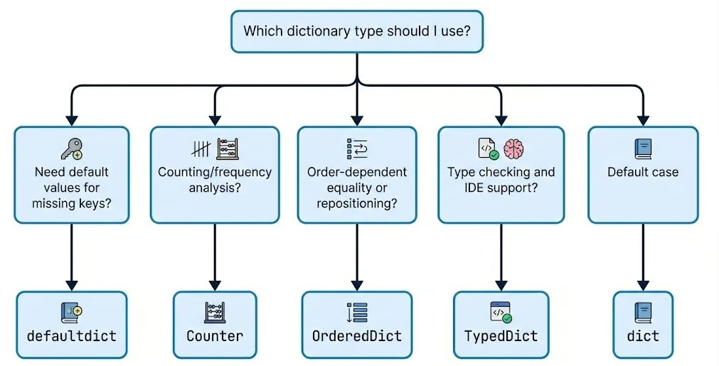
['task3', 'task1', 'task2']

The following graph illustrates when to choose which dictionary type.

Modern type safety and read-only views

As Python adoption grows in large-scale production environments, type safety becomes an important issue. The typing and types modules introduce ways to enforce structure on your dictionaries. Understanding Python dunder methods can also help you build custom dictionary-like objects with special behaviors.

TypedDict

Python's typing module provides TypedDict for defining dictionary structures with specific required keys and type annotations. This improves code documentation, enables IDE autocomplete, and catches type errors during static analysis. Let’s see how it works:

from typing import TypedDict

# Define strict structure for user data
class UserProfile(TypedDict):
    user_id: int
    username: str
    email: str
    is_active: bool
    role: str

# Create properly typed dictionary
user: UserProfile = {
    "user_id": 12345,
    "username": "data_scientist",
    "email": "scientist@company.com",
    "is_active": True,
    "role": "analyst"
}

# IDE will autocomplete and type-check
def process_user(user: UserProfile) -> str:
    # IDE knows these keys exist and their types
    return f"User {user['username']} (ID: {user['user_id']}) - {user['role']}"

# Optional keys with total=False
class PartialConfig(TypedDict, total=False):
    host: str
    port: int
    database: str  # All keys are optional

config: PartialConfig = {"host": "localhost"}  # Valid - partial config

MappingProxyType

For scenarios where you need to expose a dictionary but prevent modification, MappingProxyType creates an immutable, read-only view of a standard dictionary. This is excellent for protecting global configuration constants from accidental changes. Let’s see this in action:

from types import MappingProxyType

# Create read-only view of configuration
_INTERNAL_CONFIG = {
    "API_VERSION": "v2",
    "MAX_RETRIES": 3,
    "TIMEOUT": 30,
    "ENDPOINTS": {
        "users": "/api/v2/users",
        "data": "/api/v2/data"
    }
}

# Expose as immutable proxy
CONFIG = MappingProxyType(_INTERNAL_CONFIG)

# Reading works normally
print(CONFIG["API_VERSION"]) 
print(CONFIG["TIMEOUT"]) 

# Modifications raise TypeError
try:
    CONFIG["TIMEOUT"] = 60
except TypeError as e:
    print(f"Cannot modify: {e}")

# Caution: nested modifications succeed
try:
    CONFIG["ENDPOINTS"]["users"] = "/new/endpoint"
except TypeError as e:
    print(f"Cannot modify nested: {e}")

# Practical use case: Class constants
class DataPipeline:
    _default_config = {
        "batch_size": 1000,
        "parallel_workers": 4,
        "retry_failed": True
    }
    
    # Expose as read-only to prevent accidental changes
    DEFAULT_CONFIG = MappingProxyType(_default_config)
    
    def __init__(self, custom_config=None):
        # Merge with custom config while keeping defaults safe
        self.config = {**self.DEFAULT_CONFIG, **(custom_config or {})}

v2
30
Cannot modify: 'mappingproxy' object does not support item assignment

So, as we can see, MappingProxyType makes the dictionary itself read-only (no adding, deleting, or rebinding keys), but it does not freeze mutable values stored inside it. To prevent changes to nested structures, you must also make those nested objects immutable or wrap them in their own read-only views.

Function signatures and type hints

For function signatures and type hints, use Dict and Mapping from the typing module to document expected dictionary structures. We can do that as shown below:

from typing import Dict, List, Mapping, Any

# Dict for mutable dictionaries
def process_scores(scores: Dict[str, float]) -> Dict[str, str]:
    """Convert numeric scores to letter grades."""
    grades = {}
    for student, score in scores.items():
        if score >= 90:
            grades[student] = "A"
        elif score >= 80:
            grades[student] = "B"
        elif score >= 70:
            grades[student] = "C"
        else:
            grades[student] = "F"
    return grades

# Mapping for read-only or general mapping types
def display_config(config: Mapping[str, Any]) -> None:
    """Display configuration - accepts any mapping type."""
    for key, value in config.items():
        print(f"{key}: {value}")

# Works with dict, MappingProxyType, OrderedDict, etc.
display_config({"host": "localhost", "port": 5432})
display_config(CONFIG)  # MappingProxyType from earlier

host: localhost
port: 5432
API_VERSION: v2
MAX_RETRIES: 3
TIMEOUT: 30
ENDPOINTS: {'users': '/new/endpoint', 'data': '/api/v2/data'}

Optimizing the Performance of Python Dictionary Methods 

As your datasets grow from thousands to millions of records, the efficiency of your code becomes important. For this reason, it is necessary to understanding the performance characteristics of dictionaries. So, let's look at the computational complexity, memory implications, and optimization strategies for dictionary operations.

Time complexity analysis

Dictionary operations achieve their high speed through hash table implementation, delivering average-case O(1) time complexity for the three most common operations: 

• Retrieving values (get)
• Inserting or updating entries (set)
• Removing entries (delete)

This constant-time performance means these operations take roughly the same order of magnitude of time on average, whether your dictionary contains 10 items or 10 million. Let’s see this with a code example:

import time
import statistics


def benchmark_lookup(size, repeats=50_000):
    """
    Measure the median time for a single dictionary lookup in a dictionary of given size.
    
    Parameters:
        size (int): Number of elements in the dictionary to create
        repeats (int): How many times to repeat the lookup (for more stable median)
    
    Returns:
        float: Median lookup time in microseconds (μs)
    """
    # Create a large dictionary with string keys and integer values
    large_dict = {f"key_{i}": i for i in range(size)}
    
    # The key we will look up repeatedly (last element)
    target_key = f"key_{size - 1}"
    
    # Store individual measurement times (in nanoseconds)
    times = []
    
    # Perform many lookups to reduce measurement noise
    for _ in range(repeats):
        # Use high-resolution timer (nanoseconds)
        start = time.perf_counter_ns()
        _ = large_dict[target_key]          # The actual dictionary lookup
        end = time.perf_counter_ns()
        times.append(end - start)
    
    # Calculate median time to minimize impact of outliers
    median_ns = statistics.median(times)
    
    # Convert nanoseconds to microseconds
    return median_ns / 1000


# Sizes to test (from 100k to 10 million elements)
sizes = [100_000, 1_000_000, 10_000_000]

print("Dictionary lookup benchmark (median time over many repeats)\n")
print(f"{'Size':>12} | {'Median Lookup Time':>18} | Notes")
print("-" * 50)

for size in sizes:
    lookup_time_us = benchmark_lookup(size)
    print(f"{size:>12,} | {lookup_time_us:>15.2f} μs   | "
          f"{'→ still ~constant' if size == sizes[-1] else ''}")

Dictionary lookup benchmark (median time over many repeats)

        Size | Median Lookup Time | Notes
--------------------------------------------------
     100,000 |            0.14 μs   | 
   1,000,000 |            0.14 μs   | 
  10,000,000 |            0.14 μs   | → still ~constant

The above median lookup times can change for you based on your computational resources. The key point to be noted is that whatever may be the values they almost remain same with some variability making the difference completely negligible proving the O(1) property.

Average-case vs worst-case

However, in the worst-case scenario, it can degrade to O(n) complexity when excessive hash collisions occur. Hash collisions happen when different keys produce the same hash value, forcing Python to search through multiple entries stored at the same hash bucket. Let’s see this with an example:

# Pathological case: forcing hash collisions
class BadHash:
    """Object with intentionally poor hash function."""
    def __init__(self, value):
        self.value = value
    
    def __hash__(self):
        return 1  # All instances hash to same value - worst case!
    
    def __eq__(self, other):
        return isinstance(other, BadHash) and self.value == other.value

# This will have O(n) performance due to collisions
bad_dict = {BadHash(i): i for i in range(1000)}

# Compare with well-distributed hashes
good_dict = {f"key_{i}": i for i in range(1000)}

# Benchmark the difference
start = time.perf_counter()
_ = bad_dict[BadHash(999)]
bad_time = time.perf_counter() - start

start = time.perf_counter()
_ = good_dict["key_999"]
good_time = time.perf_counter() - start

print(f"Bad hash lookup: {bad_time * 1_000_000:.2f} μs")
print(f"Good hash lookup: {good_time * 1_000_000:.2f} μs")
print(f"Performance degradation: {bad_time / good_time:.1f}x slower")

Bad hash lookup: 582.48 μs
Good hash lookup: 93.99 μs
Performance degradation: 6.2x slower

Again, the exact results and the performance degradation will vary depending on your computational power. But the tendency will be the same: the bad hash lookup will take much longer than the one achieving O(1) time complexity.

Dictionary resizing

Another hidden cost is resizing. As dictionaries grow, Python automatically resizes the internal hash table to maintain performance. This resizing operation has a computational cost, as it requires rehashing all existing keys and redistributing them across a larger array. 

Python uses a growth factor strategy, typically at least doubling the size when a threshold is reached. Understanding these resizing patterns helps when initializing large dictionaries. If you know the approximate final size, you can pre-allocate space to avoid multiple resizing operations. 

Memory management and sizing

Speed often comes at the cost of memory. Dictionaries have a significant memory overhead compared to tuples or lists because they must store the hash table structure (indices, hashes, keys, and values). Let’s understand this with a code example:

import sys

# Compare memory footprint of different data structures
data_list = [("name", "Alice"), ("age", 30), ("city", "NYC")]
data_tuple = (("name", "Alice"), ("age", 30), ("city", "NYC"))
data_dict = {"name": "Alice", "age": 30, "city": "NYC"}

print(f"List of tuples: {sys.getsizeof(data_list)} bytes")
print(f"Tuple of tuples: {sys.getsizeof(data_tuple)} bytes")
print(f"Dictionary: {sys.getsizeof(data_dict)} bytes")

List of tuples: 88 bytes
Tuple of tuples: 64 bytes
Dictionary: 184 bytes

Using __slots__ to reduce object size

In the above example, you can see that the dictionary uses ~2x-3x more memory for the same data. For classes that create many instances, using __slots__ instead of instance __dict__ can dramatically reduce memory consumption. 

By default, Python stores instance attributes in a dictionary accessible via __dict__, but __slots__ uses a more compact array-based structure. Let’s see an example of this:

import sys

# Regular class - uses __dict__ for attributes
class RegularUser:
    def __init__(self, user_id, name, email):
        self.user_id = user_id
        self.name = name
        self.email = email

# Optimized class - uses __slots__
class OptimizedUser:
    __slots__ = ['user_id', 'name', 'email']
    
    def __init__(self, user_id, name, email):
        self.user_id = user_id
        self.name = name
        self.email = email

# Create instances
regular = RegularUser(12345, "Alice", "alice@example.com")
optimized = OptimizedUser(12345, "Alice", "alice@example.com")

# Compare memory usage
print(f"Regular instance: {sys.getsizeof(regular.__dict__)} bytes (__dict__)")
print(f"Optimized instance: {sys.getsizeof(optimized)} bytes (__slots__)")

# For massive instance counts, the savings multiply
regular_users = [RegularUser(i, f"User{i}", f"user{i}@example.com") for i in range(1000)]
optimized_users = [OptimizedUser(i, f"User{i}", f"user{i}@example.com") for i in range(1000)]

regular_total = sum(sys.getsizeof(u.__dict__) for u in regular_users)
optimized_total = sum(sys.getsizeof(u) for u in optimized_users)

print(f"\n1000 regular instances: {regular_total:,} bytes")
print(f"1000 optimized instances: {optimized_total:,} bytes")
print(f"Memory savings: {((regular_total - optimized_total) / regular_total * 100):.1f}%")

Regular instance: 296 bytes (__dict__)
Optimized instance: 56 bytes (__slots__)

1000 regular instances: 96,000 bytes
1000 optimized instances: 56,000 bytes
Memory savings: 41.7%

Python dictionary vs pandas DataFrame

Finally, while dictionaries are excellent for random access, they are not optimized for columnar data processing. If you are handling large-scale tabular data (e.g., millions of rows), migrating to a pandas DataFrame is a wise choice, because they are optimized for both memory efficiency and vectorized speed. 

import pandas as pd
import time
import sys

n = 10_000

# Dict
dict_data = {i: {"user_id": i, "score": i * 1.5, "category": f"cat_{i % 10}"} for i in range(n)}

# Optimized DF: use category dtype for strings, int32 for ids
df_data = pd.DataFrame({
    "user_id": pd.Series(range(n), dtype="int32"),
    "score": [i * 1.5 for i in range(n)],
    "category": pd.Series([f"cat_{i % 10}" for i in range(n)], dtype="category")
})

dict_memory = sys.getsizeof(dict_data)
df_memory = df_data.memory_usage(deep=True).sum()

print(f"Dictionary: {dict_memory:,} bytes")
print(f"Optimized DataFrame: {df_memory:,} bytes")

# Bulk operation: mean score per category
start = time.perf_counter()
df_mean = df_data.groupby("category")["score"].mean()
df_time = (time.perf_counter() - start) * 1_000_000

# Equivalent in dict (manual loop)
start = time.perf_counter()
from collections import defaultdict
means = defaultdict(lambda: [0, 0])
for row in dict_data.values():
    cat = row["category"]
    means[cat][0] += row["score"]
    means[cat][1] += 1
dict_mean = {k: s/c for k, (s, c) in means.items()}
dict_time = (time.perf_counter() - start) * 1_000_000

print(f"\nDF groupby mean: {df_time:.2f} μs")
print(f"Dict manual mean: {dict_time:.2f} μs")

Dictionary: 294,992 bytes
Optimized DataFrame: 130,972 bytes

DF groupby mean: 1630.24 μs
Dict manual mean: 3931.47 μs

You can clearly see that the DataFrame outperforms the dictionary in our example. For data science workflows that require both fast lookups and analytical operations, consider hybrid approaches like using dictionaries for indexing and quick access, then convert to DataFrames for bulk analysis. 

The key to optimization is matching the data structure to your access patterns. If you're doing frequent key-based lookups, dictionaries are optimal. For columnar operations, filtering, and aggregations on large datasets, DataFrames provide good performance. 

Conclusion

Dictionaries are far more than simple storage containers. They are the glue that holds complex data science applications together. If you are building a quick lookup table for a script or architecting a high-throughput data pipeline, then a dictionary is likely your most valuable tool.

However, relying on default behavior without robust error handling is a recipe for runtime failure. Robust error handling patterns, like using EAFP versus LBYL approaches and proactive validation, are likely to prevent runtime failures when processing external data. 

Specialized collections like defaultdict, Counter, and TypedDict make your code go from functional to production-grade. Always keep time complexity and memory management in mind to make sure your code runs efficiently. Also, remember that optimization is an iterative process.

To continue building your Python skills, I recommend taking our Intermediate Python course for more on data structures, or the broader Python Developer career track for a comprehensive learning path.