Most LLM apps are full of small decisions: Which tool should the agent call? Which model should handle this query? Does this message break a policy?
Today, many teams answer these questions by asking a generative model to write the answer as text, then parsing that text to make a decision.
Google's Gemini Decisions API takes a different approach. It uses the Gemini Decision 1 model to score a fixed set of options in a single forward pass and returns a probability for each option, with zero output tokens billed.
In this tutorial, we'll run the same intent classification task on two setups:
- Gemini Decision 1 through the Decisions API
- Gemini 3.5 Flash-Lite through the Interactions API, using structured JSON output
We'll compare them on accuracy, latency, token usage, cost, and calibration, and then push both from 1 to 100 questions in a single request.
By the end of this tutorial, you'll know how to:
-
Call the Decisions API with choice questions and read its probabilities and confidence scores
-
Build a generative baseline with the Interactions API and a JSON schema
-
Measure latency, token usage, and cost for both approaches
-
Check whether a model's confidence can be trusted, using a reliability diagram and expected calibration error (ECE)
-
Decide when a decision model fits your app better than a generative one
You can run the complete code in this Google Colab.
Decision Models vs. Generative Models
Before we look at how each one works, let's define the two terms.
- Generative model: This model produces new content. You give it a prompt, and it writes a response one token at a time. That response can be anything like an answer, a summary, code, or a label. Gemini 3.5 Flash-Lite, like most LLMs we use in chat apps, is a generative model.
- Decision model: A decision model picks from the options you define. You give it an input and a fixed list of possible answers, and it tells you the probability of each option without writing a single line of text. Gemini Decision 1 is a decision model.
Here's an example.
A customer writes to a bank: "My card hasn't arrived yet. When will it come?"
If you ask a generative model, "What does this customer want?", it might reply:
“The customer is waiting for a new card and wants to know when it will arrive.”
That's a good answer for a human to read. But if your app needs to route the message to the right team, your code now has to turn that sentence into a label. You can force a label with a JSON schema, but the model still writes it token by token.
However, if you ask a decision model the same thing, you first give it the options, such as card_arrival, lost_or_stolen_card, and exchange_rate. It returns a probability for each one:
card_arrival         0.91
lost_or_stolen_card  0.06
exchange_rate        0.03
Your code can then act on that probability directly by routing to the card team if card_arrival is above a threshold, and sending it to a human if not. In short:
| |
Generative model
|
Decision model
|
|
Returns
|
Text it writes
|
A probability for each option you define
|
|
Possible answers
|
Open ended
|
Fixed set
|
|
Good for
|
Answers, summaries, explanations, and extraction
|
Routing, tool selection, policy checks, and grading
|
In practice, many apps use a generative model for both jobs. That’s what we’ll test in the next section: whether a decision model does the classification part better than a generative model.
When you use a generative model as a classifier, it writes the answer one token at a time. For a JSON answer like ours, the output looks like this as it is generated:
{
{"intent":
{"intent": "card_arrival",
{"intent": "card_arrival", "confidence": 0.95}
Each token is a separate decoding step, and each output token is billed. If you want a confidence score, the model has to write that number too. That number is the model's own guess about itself, not a probability measured from its internals.
A decision model, however, skips this writing step. You give it the options up front, and it scores all of them against the input in one forward pass. The result is a probability for every option:
card_arrival            0.12
card_delivery_estimate  0.85
lost_or_stolen_card     0.01
...
This changes three things you can measure:
- Latency: There is no decoding loop, so latency should not grow with the length of the answer.
- Cost: There are no output tokens to bill. You pay only for input tokens, which include your question text and option descriptions.
- Confidence: The confidence comes from the probabilities themselves, so it should track how often the model is right.
The trade-off is that you can only ask closed-set questions. A decision model can't explain its answer, extract a value, or write free text.
Demo: Building a Banking Intent Classifier
In this demo, we’ll build a banking intent classifier. We'll use the test split of Banking77, a public dataset of customer messages labeled with 77 intents, and keep 12 intents that are easy to confuse with each other:
-
card_arrival and card_delivery_estimate
-
pending_card_payment, declined_card_payment, and card_payment_fee_charged
-
pending_transfer, transfer_not_received_by_recipient, and balance_not_updated_after_bank_transfer
-
lost_or_stolen_card, card_not_working, exchange_rate, and top_up_failed
Similar intents make the task harder, which makes the confidence scores more interesting to study.
We'll run the classifier with both models in two ways:
- One message per request: 180 messages (15 per intent), sent to each model one at a time.
- Many questions per request: N messages placed in one shared input, with one question per message, for N = 1, 5, 10, 25, 50, and 100.
Here are the settings we keep the same for both models:
|
Setting
|
Value used
|
Why
|
|
Decision model
|
gemini-decision-1
|
The model under test
|
|
Generative model
|
gemini-3.5-flash-lite
|
The cost-efficient generative baseline used in the launch post comparison
|
|
Flash-Lite temperature
|
0.0
|
Removes sampling noise from the baseline
|
|
Flash-Lite thinking level
|
minimal
|
Keeps the comparison about decoding, not reasoning
|
|
Output format
|
JSON schema with an enum of the 12 labels
|
Flash-Lite can only return a valid label
|
|
Option descriptions
|
One short sentence per intent
|
Both models see the same label definitions
|
|
Warmup calls
|
2 per model
|
Keeps the connection setup out of the measurements
|
|
Repeats (many questions per request)
|
3 per setting
|
We report the median, not a single run
|
Note: These are working settings for this demo, not tuned settings for either model.
Step 1: Prerequisites and setup
To follow along, you need:
-
A Gemini API key from Google AI Studio
-
A Colab notebook (or any Python 3 environment)
-
google-genai version 3.2 or later
The Decisions API has a no-cost tier in Google AI Studio for prototyping, so you can try it before paying. I ran this demo in Colab, but feel free to use any Python 3 environment.
Let’s start by installing the packages:
!pip install -q -U "google-genai>=3.2" pandas matplotlib
Here, google-genai is Google's Python SDK for the Gemini API. It gives us the client.decisions.create and client.interactions.create methods, which send requests to the Decisions API and the Interactions API. We use pandas to load the dataset and organize results, and matplotlib to plot the figures.
Next, we create the client. The Decisions API needs the v1beta API version:
import os, time, json
import numpy as np
import pandas as pd
from google import genai
client = genai.Client(
    api_key=os.environ["GEMINI_API_KEY"],
    http_options={"api_version": "v1beta"},
)

DECISION_MODEL = "gemini-decision-1"
GEN_MODEL = "gemini-3.5-flash-lite"
Here, genai.Client() reads the API key from the GEMINI_API_KEY set under the secrets in Colab or as an environment variable, and http_options points it at the v1beta API, where the Decisions API lives.
Then we’ll load the Banking77 dataset and define our 12 intents. Each intent gets a one-sentence description that both models will see:
BANKING77_URL = (
"https://raw.githubusercontent.com/PolyAI-LDN/task-specific-datasets/master/banking_data/test.csv"
)
INTENTS = {
"card_arrival": "The customer is asking where their new card is or why it has not arrived yet.",
"card_delivery_estimate": "The customer wants to know how long card delivery usually takes.",
"lost_or_stolen_card": "The customer's card was lost or stolen.",
}
LABELS = list(INTENTS)
df = pd.read_csv(BANKING77_URL)
df = df[df["category"].isin(LABELS)].reset_index(drop=True)
sample = (
df.groupby("category")
.sample(n=15, random_state=42)
.sample(frac=1, random_state=42)
.reset_index(drop=True)
)
The above code snippet downloads the Banking77 test split as a CSV file and keeps only the rows labeled with one of our 12 intents. It then samples 15 messages per intent with a fixed random seed, so you get the same sample on every run. The final .sample(frac=1) shuffles the rows so the intents are mixed.
This gives us 180 messages, 15 per intent.
Step 2: Classify with the Decisions API
A choice question takes a dictionary that maps each option ID to a description. We pass the message as input and ask one question, keyed intent:
def decide_intent(text):
    start = time.perf_counter()
    result = client.decisions.create(
        model=DECISION_MODEL,
        input=text,
        questions={
            "intent": {
                "type": "choice",
                "instructions": "Which intent best describes this banking customer message?",
                "criteria": INTENTS,
            }
        },
    )
    latency = time.perf_counter() - start
    ans = result.answers["intent"]
    return {
        "pred": ans.choice,
        "confidence": float(ans.confidence),
        "probabilities": dict(ans.probabilities),
        "latency_s": latency,
        "input_tokens": result.usage.total_input_tokens,
        "output_tokens": result.usage.total_output_tokens,
    }
The decide_intent() function sends one message as the input and one choice question with our 12 intents as options. We time the call with time.perf_counter(), then read the top choice, confidence, all option probabilities, and token counts from the response.
Each answer carries three fields:
-
choice: The option with the highest probability
-
probabilities: One probability per option, summing to 1
-
confidence: The estimated probability that the top answer is correct
The usage object reports input tokens, and total_output_tokens is always 0.
Here's the result for the first message in our sample:
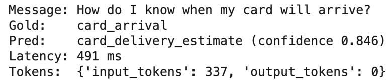
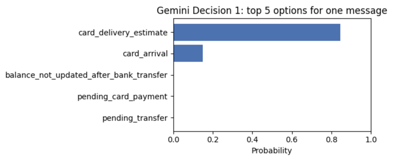
The model confused two similar intents, but its confidence of 0.846 shows some uncertainty. The good part is that the correct intent, card_arrival, came second with almost all of the remaining probability (about 0.15). All other options were close to zero.
Step 3: Classify with Flash-Lite
For the generative baseline, we use structured output with an enum of the same 12 labels, so Flash-Lite can only return a valid label. We also ask for a confidence between 0 and 1, which is how most apps get a confidence score from a generative model:
LABEL_LIST = "\n".join(f"- {k}: {v}" for k, v in INTENTS.items())

GEN_SCHEMA = {
    "type": "object",
    "properties": {
        "intent": {"type": "string", "enum": LABELS},
        "confidence": {"type": "number"},
    },
    "required": ["intent", "confidence"],
}

def generate_intent(text):
    prompt = (
        "Which intent best describes this banking customer message?\n\n"
        f"Intents:\n{LABEL_LIST}\n\n"
        f"Message: {text}\n\n"
        "Return the intent and your confidence from 0 to 1."
    )
    start = time.perf_counter()
    interaction = client.interactions.create(
        model=GEN_MODEL,
        input=prompt,
        response_format={
            "type": "text",
            "mime_type": "application/json",
            "schema": GEN_SCHEMA,
        },
        generation_config={"temperature": 0.0, "thinking_level": "minimal"},
        store=False,
    )
    latency = time.perf_counter() - start
    parsed = json.loads(interaction.output_text)
    return {
        "pred": parsed["intent"],
        "confidence": float(parsed["confidence"]),
        "latency_s": latency,
        "input_tokens": interaction.usage.total_input_tokens,
        "output_tokens": interaction.usage.total_output_tokens,
        "thought_tokens": interaction.usage.total_thought_tokens,
    }
The generate_intent() function builds a prompt with the 12 intents and their descriptions. It calls Flash-Lite with response_format set to our JSON schema, so the output must be valid JSON with one of the 12 labels. Temperature is set to 0 with minimal thinking level to keep the answer stable and short. We then parse interaction.output_text with json.loads() and read the token counts from interaction.usage.
I tested the same message as in the previous step with Flash-Lite, and it made the same mistake with higher confidence:
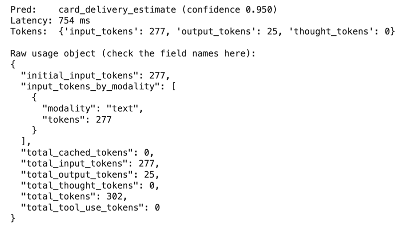
Thinking tokens are 0, which confirms that minimal thinking kept Flash-Lite to writing the answer only. Flash-Lite used fewer input tokens than Decision 1 (277 vs 337) because the Decisions API counts the option descriptions inside the question as input.
Step 4: Classify one message per request
Now, let's send all 180 messages to both models, one request at a time, after two warmup calls each:
rows = []
for i, r in sample.iterrows():
    for model_name, fn in (("decision", decide_intent), ("generative", generate_intent)):
        out = fn(r["text"])
        rows.append({
            "model": model_name, "gold": r["category"], "pred": out["pred"],
            "confidence": out["confidence"], "latency_s": out["latency_s"],
            "input_tokens": out["input_tokens"], "output_tokens": out["output_tokens"],
        })

exp1 = pd.DataFrame(rows)
exp1["correct"] = exp1["pred"] == exp1["gold"]
This loop sends each message to both functions and saves the prediction, confidence, latency, and token counts as one row. We then turn the rows into a DataFrame and add a correct column that marks whether each prediction matches the true label.
Here are the results:
|
Metric
|
Gemini Decision 1
|
Gemini 3.5 Flash-Lite
|
|
Accuracy
|
84.4%
|
83.9%
|
|
Median latency
|
325 ms
|
1,068 ms
|
|
p90 latency
|
412 ms
|
6,483 ms
|
|
Slowest request
|
1.0 s
|
101.6 s
|
|
Requests over 5 s
|
0 of 180
|
33 of 180
|
|
Mean input tokens
|
339
|
279
|
|
Mean output tokens
|
0
|
25
|
Here are three things we learned from these metrics:
- Accuracy: Both models were about equally accurate.
- Latency: Decision 1 was about 3x faster at the median and much more consistent, while Flash-Lite had a long tail of slow requests.
- Tokens: Decision 1 used more input tokens because the option descriptions count as input, but it generated no output tokens.
Note: Our timing includes the network round-trip from Colab, so treat that gap as setup-dependent.
Step 5: Check calibration
Accuracy tells us how often a model is right, but calibration tells us whether its confidence means anything or not. A model is well calibrated when its confidence matches its accuracy, i.e., if it says 0.8 on a group of answers, about 80% of them should be correct.
To measure this, we group predictions into 10 confidence bins and compare each bin's average confidence with its accuracy. Expected calibration error (ECE) is the average gap, weighted by how many predictions fall in each bin. Lower is better.
def ece(conf, correct, n_bins=10):
    conf = np.asarray(conf, dtype=float)
    correct = np.asarray(correct, dtype=float)
    edges = np.linspace(0, 1, n_bins + 1)
    ids = np.clip(np.digitize(conf, edges[1:-1]), 0, n_bins - 1)
    total = 0.0
    for b in range(n_bins):
        mask = ids == b
        if mask.sum():
            total += mask.mean() * abs(conf[mask].mean() - correct[mask].mean())
    return total
The ece() function places each prediction into one of 10 bins by its confidence (0 to 0.1, 0.1 to 0.2, and so on). For each bin, it takes the gap between average confidence and accuracy, weights it by the share of predictions in that bin, and adds up the results.
Here's how the two models compare:
|
Metric
|
Gemini Decision 1
|
Gemini 3.5 Flash-Lite
|
|
Accuracy
|
84.4%
|
83.9%
|
|
Mean confidence
|
0.867
|
0.957
|
|
ECE
|
0.050
|
0.124
|
|
Mean confidence when correct
|
0.901
|
0.966
|
|
Mean confidence when wrong
|
0.686
|
0.912
|
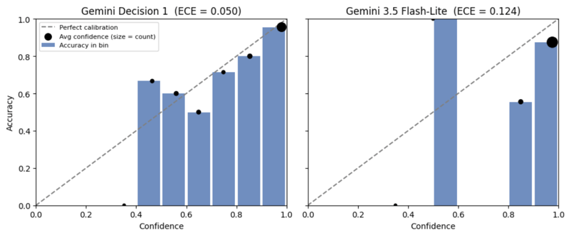
Figure: Reliability diagrams for both models
Decision 1's confidence is close to its accuracy, with an ECE of 0.050. It is also clearly lower when the model is wrong (0.686) than when it is right (0.901).
Flash-Lite is overconfident. It reports 0.957 on average while being right 83.9% of the time. It used only 9 distinct confidence values across 180 answers, and 158 of them were 0.95 or higher. Even its wrong answers averaged 0.912. The number looks like a probability, but it is the model's own estimate written as text.
Calibration matters when you act on the score. A common pattern is to accept answers above a confidence threshold and send the rest to a fallback model or a human:
|
Threshold
|
Decision 1: share kept
|
Decision 1: accuracy on kept
|
Flash-Lite: share kept
|
Flash-Lite: accuracy on kept
|
|
0.50
|
94.4%
|
85.9%
|
99.4%
|
84.4%
|
|
0.70
|
78.3%
|
92.2%
|
98.9%
|
84.3%
|
|
0.80
|
74.4%
|
93.3%
|
98.9%
|
84.3%
|
|
0.90
|
63.3%
|
95.6%
|
88.9%
|
87.5%
|
|
0.95
|
53.9%
|
96.9%
|
87.8%
|
87.3%
|
With Decision 1, a higher threshold works as expected. At 0.9, it keeps 63% of messages at 95.6% accuracy. With Flash-Lite, the threshold barely helps, because most of its wrong answers also have high confidence. The official docs recommend choosing a threshold from labeled examples of your own traffic.
Step 6: Classify 100 messages in one request
The Decisions API can answer up to 1,000 questions about one shared input in a single request. To test this, we put N customer messages into one input and ask one question per message.
For Decision 1, that means N choice questions keyed m1 to mN:
def build_batch(n):
    msgs = pool.iloc[:n]
    shared = "Banking customer messages:\n" + "".join(
        f"Message {i + 1}: {t}\n" for i, t in enumerate(msgs["text"])
    )
    return shared, list(msgs["category"])

def decide_batch(n):
    shared, gold = build_batch(n)
    questions = {
        f"m{i + 1}": {
            "type": "choice",
            "instructions": f"Which intent best describes Message {i + 1}?",
            "criteria": INTENTS,
        }
        for i in range(n)
    }
    result = client.decisions.create(
        model=DECISION_MODEL, input=shared, questions=questions
    )
    preds = [result.answers[f"m{i + 1}"].choice for i in range(n)]
    return preds, gold, result.usage
Here, the build_batch() function numbers the first N messages and joins them into one shared input. Then decide_batch() creates one choice question per message, keyed m1 to mN, sends them all in a single request, and reads back one answer per key.
For Flash-Lite, we send the same shared input with a JSON schema that has N fields, each limited to 12 labels. Each N uses the same messages for both models, and each setting runs three times.
|
Questions per request
|
Decision 1: median latency
|
Flash-Lite: median latency
|
Decision 1: input tokens
|
Flash-Lite: input / output tokens
|
|
1
|
318 ms
|
888 ms
|
344
|
291 / 14
|
|
5
|
353 ms
|
858 ms
|
1,554
|
369 / 64
|
|
10
|
398 ms
|
1,063 ms
|
3,056
|
456 / 129
|
|
25
|
546 ms
|
2,753 ms
|
7,570
|
710 / 350
|
|
50
|
592 ms
|
Failed
|
15,100
|
Failed
|
|
100
|
59,095 ms
|
Failed
|
30,309
|
Failed
|
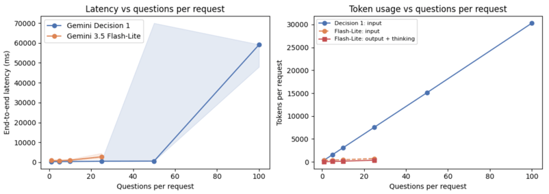
Up to 25 questions, Decision 1's median latency stayed under 550 ms. Flash-Lite's median grew with N, from under 1s at 1 to 5 questions to 2.75 s at 25, because it has to write every answer as output tokens. Even at 50 questions, Decision 1's median was 592 ms, though one of the three runs took 70 s.
Here are two key points to ponder:
- Flash-Lite failed at 50 and 100 questions: The "Failed" rows in the table above are all the same 400 error. It shows that the schema "has too many states for serving." A schema with 50 or more fields, each limited to 12 labels, is more than the API accepts.
- Decision 1 slowed down at 100 questions: Each question repeats all 12 option descriptions, about 300 tokens per question, so the request reached 30,309 tokens, while Google's flat latency claim covers contexts up to 16K tokens.
Step 7: Trim the requests
Now, an obvious question arises: can we fix the slowdown and the failures? For Decision 1, we use empty option descriptions (""). For Flash-Lite, we ask for one list of N labels instead of N separate fields:
"criteria": {k: "" for k in LABELS}
schema = {
"type": "object",
"properties": {"intents": {
"type": "array",
"items": {"type": "string", "enum": LABELS},
"minItems": n, "maxItems": n,
}},
"required": ["intents"],
}
Here's how Decision 1 did with empty descriptions:
|
Questions per request
|
Median latency
|
Accuracy
|
Input tokens
|
|
25
|
357 ms
|
84.0%
|
3,995
|
|
50
|
649 ms
|
78.0%
|
7,950
|
|
100
|
1,603 ms
|
83.0%
|
16,009
|
Dropping the descriptions roughly halved the input tokens. At 100 questions, the request came down to about 16K tokens, and median latency fell from 59 s to 1.6 s. Accuracy dropped a little at 25 and 50 questions, so short descriptions are a better middle ground than none, especially for similar intents.
The list schema didn't help the Flash-Lite model. It worked at 25 questions, but still failed at 50 and 100.
Step 8: Compare cost
Finally, we compute the cost from the token counts each API returns, using paid-tier prices:
|
Model
|
Input price per 1M tokens
|
Output price per 1M tokens
|
|
Gemini Decision 1
|
$0.10
|
$0
|
|
Gemini 3.5 Flash-Lite
|
$0.30
|
$2.50 (including thinking tokens)
|
def cost_per_request(model, input_tokens, output_tokens, thought_tokens):
    if model == "decision":
        return input_tokens * 0.10 / 1e6
    return (input_tokens * 0.30 + (output_tokens + thought_tokens) * 2.50) / 1e6
The cost_per_request() function multiplies each token count by its price per 1M tokens. For Decision 1, only input tokens count. For Flash-Lite, thinking tokens are billed at the output price, so we add them to the output tokens.
Here's the cost per 1,000 requests for each setup:
|
Setup
|
Gemini Decision 1
|
Gemini 3.5 Flash-Lite
|
Flash-Lite / Decision 1
|
|
1 message per request
|
$0.034
|
$0.147
|
4.3x
|
|
5 questions per request
|
$0.155
|
$0.271
|
1.7x
|
|
10 questions per request
|
$0.306
|
$0.459
|
1.5x
|
|
25 questions per request
|
$0.757
|
$1.088
|
1.4x
|
|
25 questions, trimmed setups (Step 7)
|
$0.400
|
$0.831
|
2.1x
|
|
50 questions per request
|
$1.510
|
Failed
|
n/a
|
|
100 questions, empty descriptions
|
$1.601
|
Failed
|
n/a
|
On single messages, Decision 1 was 4.3x cheaper, but the gap shrinks as you batch more questions into one request. The shared input is billed once in both APIs. But each Decision 1 question carries its own instruction and all 12 option descriptions, while Flash-Lite sees the label list only once and pays for a short output per answer. At 25 questions, Decision 1 used 7,570 input tokens against Flash-Lite's 710 input and 350 output tokens.
Note: The Decisions API doesn't support context caching or the Batch API. If you send the same input in several requests, it is billed in full each time. So when you have many questions about the same input, ask them in one request rather than spreading them across calls.
When to Use Each Approach
Based on the above runs, a decision model is the better fit when:
- The answer comes from a fixed set of options, like intents, routes, tools, or policy labels
- The decision sits in the request path, where every user waits for it
- You want to act on confidence, like, by sending unclear cases to a fallback or a human
- You need to ask many independent questions about the same input in one request
A generative model is still the better fit when:
- You need an explanation, an extracted value, or any free text
- The set of possible answers is open or changes per request
- You already made a generative call on that input and can add the classification to it
|
Use the Decisions API when you need
|
Use the Interactions API when you need
|
|
A yes/no probability, one option from a fixed set, or a rating on a fixed scale
|
Generated text, summaries, or explanations
|
|
Calibrated probabilities that you can threshold
|
Extracted values or objects that follow your own JSON schema
|
|
Many independent checks over the same input in one call
|
Tool calls with arguments
|
|
Low latency and zero output token cost
|
Multi-step reasoning
|
Final Thoughts
In this tutorial, we built a banking intent classifier with Gemini Decision 1 and Gemini 3.5 Flash-Lite, then calculated accuracy, latency, calibration, and cost to compare the two models. Here are four takeaways from the tutorial:
- Accuracy was a tie: 84.4% for Decision 1 and 83.9% for Flash-Lite, with the same verdict on 163 of 180 messages.
- Decision 1 was faster and more predictable: Its median latency was 325 ms against 1,068 ms, and its slowest request took 1.0 s against 101.6 s.
- Decision 1's confidence was usable: Its ECE was 0.050 against 0.124, and raising the threshold to 0.9 lifted accuracy on kept answers from 84.4% to 95.6%. Flash-Lite's self-reported confidence barely separated right answers from wrong ones.
- Cost and scaling depend on how you write the questions: Decision 1 was 4.3x cheaper on single messages, but every question pays for its option descriptions. So, keep the total input under about 16K tokens and keep option descriptions short.
These results come from one task, one dataset, and a small number of runs from a Colab notebook. You can treat them as observations from a demo rather than general performance claims.










Most LLM apps are full of small decisions: Which tool should the agent call? Which model should handle this query? Does this message break a policy?
Today, many teams answer these questions by asking a generative model to write the answer as text, then parsing that text to make a decision.
Google's Gemini Decisions API takes a different approach. It uses the Gemini Decision 1 model to score a fixed set of options in a single forward pass and returns a probability for each option, with zero output tokens billed.
In this tutorial, we'll run the same intent classification task on two setups:
We'll compare them on accuracy, latency, token usage, cost, and calibration, and then push both from 1 to 100 questions in a single request.
By the end of this tutorial, you'll know how to:
Call the Decisions API with
choicequestions and read its probabilities and confidence scoresBuild a generative baseline with the Interactions API and a JSON schema
Measure latency, token usage, and cost for both approaches
Check whether a model's confidence can be trusted, using a reliability diagram and expected calibration error (ECE)
Decide when a decision model fits your app better than a generative one
You can run the complete code in this Google Colab.
Decision Models vs. Generative Models
Before we look at how each one works, let's define the two terms.
Here's an example.
A customer writes to a bank: "My card hasn't arrived yet. When will it come?"
If you ask a generative model, "What does this customer want?", it might reply:
“The customer is waiting for a new card and wants to know when it will arrive.”
That's a good answer for a human to read. But if your app needs to route the message to the right team, your code now has to turn that sentence into a label. You can force a label with a JSON schema, but the model still writes it token by token.
However, if you ask a decision model the same thing, you first give it the options, such as
card_arrival,lost_or_stolen_card, andexchange_rate. It returns a probability for each one:Your code can then act on that probability directly by routing to the card team if
card_arrivalis above a threshold, and sending it to a human if not. In short:Generative model
Decision model
Returns
Text it writes
A probability for each option you define
Possible answers
Open ended
Fixed set
Good for
Answers, summaries, explanations, and extraction
Routing, tool selection, policy checks, and grading
In practice, many apps use a generative model for both jobs. That’s what we’ll test in the next section: whether a decision model does the classification part better than a generative model.
When you use a generative model as a classifier, it writes the answer one token at a time. For a JSON answer like ours, the output looks like this as it is generated:
Each token is a separate decoding step, and each output token is billed. If you want a confidence score, the model has to write that number too. That number is the model's own guess about itself, not a probability measured from its internals.
A decision model, however, skips this writing step. You give it the options up front, and it scores all of them against the input in one forward pass. The result is a probability for every option:
This changes three things you can measure:
The trade-off is that you can only ask closed-set questions. A decision model can't explain its answer, extract a value, or write free text.
Demo: Building a Banking Intent Classifier
In this demo, we’ll build a banking intent classifier. We'll use the test split of Banking77, a public dataset of customer messages labeled with 77 intents, and keep 12 intents that are easy to confuse with each other:
card_arrivalandcard_delivery_estimatepending_card_payment,declined_card_payment, andcard_payment_fee_chargedpending_transfer,transfer_not_received_by_recipient, andbalance_not_updated_after_bank_transferlost_or_stolen_card,card_not_working,exchange_rate, andtop_up_failedSimilar intents make the task harder, which makes the confidence scores more interesting to study.
We'll run the classifier with both models in two ways:
Here are the settings we keep the same for both models:
Setting
Value used
Why
Decision model
gemini-decision-1The model under test
Generative model
gemini-3.5-flash-liteThe cost-efficient generative baseline used in the launch post comparison
Flash-Lite temperature
0.0
Removes sampling noise from the baseline
Flash-Lite thinking level
minimalKeeps the comparison about decoding, not reasoning
Output format
JSON schema with an
enumof the 12 labelsFlash-Lite can only return a valid label
Option descriptions
One short sentence per intent
Both models see the same label definitions
Warmup calls
2 per model
Keeps the connection setup out of the measurements
Repeats (many questions per request)
3 per setting
We report the median, not a single run
Note: These are working settings for this demo, not tuned settings for either model.
Step 1: Prerequisites and setup
To follow along, you need:
A Gemini API key from Google AI Studio
A Colab notebook (or any Python 3 environment)
google-genaiversion 3.2 or laterThe Decisions API has a no-cost tier in Google AI Studio for prototyping, so you can try it before paying. I ran this demo in Colab, but feel free to use any Python 3 environment.
Let’s start by installing the packages:
Here,
google-genaiis Google's Python SDK for the Gemini API. It gives us theclient.decisions.createandclient.interactions.createmethods, which send requests to the Decisions API and the Interactions API. We usepandasto load the dataset and organize results, andmatplotlibto plot the figures.Next, we create the client. The Decisions API needs the v1beta API version:
Here,
genai.Client()reads the API key from theGEMINI_API_KEYset under the secrets in Colab or as an environment variable, andhttp_optionspoints it at the v1beta API, where the Decisions API lives.Then we’ll load the Banking77 dataset and define our 12 intents. Each intent gets a one-sentence description that both models will see:
The above code snippet downloads the Banking77 test split as a CSV file and keeps only the rows labeled with one of our 12 intents. It then samples 15 messages per intent with a fixed random seed, so you get the same sample on every run. The final
.sample(frac=1)shuffles the rows so the intents are mixed.This gives us 180 messages, 15 per intent.
Step 2: Classify with the Decisions API
A
choicequestion takes a dictionary that maps each option ID to a description. We pass the message asinputand ask one question, keyedintent:The
decide_intent()function sends one message as theinputand onechoicequestion with our 12 intents as options. We time the call withtime.perf_counter(), then read the top choice, confidence, all option probabilities, and token counts from the response.Each answer carries three fields:
choice: The option with the highest probabilityprobabilities: One probability per option, summing to 1confidence: The estimated probability that the top answer is correctThe
usageobject reports input tokens, andtotal_output_tokensis always 0.Here's the result for the first message in our sample:
The model confused two similar intents, but its confidence of 0.846 shows some uncertainty. The good part is that the correct intent,
card_arrival, came second with almost all of the remaining probability (about 0.15). All other options were close to zero.Step 3: Classify with Flash-Lite
For the generative baseline, we use structured output with an
enumof the same 12 labels, so Flash-Lite can only return a valid label. We also ask for a confidence between 0 and 1, which is how most apps get a confidence score from a generative model:The
generate_intent()function builds a prompt with the 12 intents and their descriptions. It calls Flash-Lite withresponse_formatset to our JSON schema, so the output must be valid JSON with one of the 12 labels. Temperature is set to0withminimalthinking level to keep the answer stable and short. We then parseinteraction.output_textwithjson.loads()and read the token counts frominteraction.usage.I tested the same message as in the previous step with Flash-Lite, and it made the same mistake with higher confidence:
Thinking tokens are 0, which confirms that
minimalthinking kept Flash-Lite to writing the answer only. Flash-Lite used fewer input tokens than Decision 1 (277 vs 337) because the Decisions API counts the option descriptions inside the question as input.Step 4: Classify one message per request
Now, let's send all 180 messages to both models, one request at a time, after two warmup calls each:
This loop sends each message to both functions and saves the prediction, confidence, latency, and token counts as one row. We then turn the rows into a DataFrame and add a correct column that marks whether each prediction matches the true label.
Here are the results:
Metric
Gemini Decision 1
Gemini 3.5 Flash-Lite
Accuracy
84.4%
83.9%
Median latency
325 ms
1,068 ms
p90 latency
412 ms
6,483 ms
Slowest request
1.0 s
101.6 s
Requests over 5 s
0 of 180
33 of 180
Mean input tokens
339
279
Mean output tokens
0
25
Here are three things we learned from these metrics:
Note: Our timing includes the network round-trip from Colab, so treat that gap as setup-dependent.
Step 5: Check calibration
Accuracy tells us how often a model is right, but calibration tells us whether its confidence means anything or not. A model is well calibrated when its confidence matches its accuracy, i.e., if it says 0.8 on a group of answers, about 80% of them should be correct.
To measure this, we group predictions into 10 confidence bins and compare each bin's average confidence with its accuracy. Expected calibration error (ECE) is the average gap, weighted by how many predictions fall in each bin. Lower is better.
The
ece()function places each prediction into one of 10 bins by its confidence (0 to 0.1, 0.1 to 0.2, and so on). For each bin, it takes the gap between average confidence and accuracy, weights it by the share of predictions in that bin, and adds up the results.Here's how the two models compare:
Metric
Gemini Decision 1
Gemini 3.5 Flash-Lite
Accuracy
84.4%
83.9%
Mean confidence
0.867
0.957
ECE
0.050
0.124
Mean confidence when correct
0.901
0.966
Mean confidence when wrong
0.686
0.912
Figure: Reliability diagrams for both models
Decision 1's confidence is close to its accuracy, with an ECE of 0.050. It is also clearly lower when the model is wrong (0.686) than when it is right (0.901).
Flash-Lite is overconfident. It reports 0.957 on average while being right 83.9% of the time. It used only 9 distinct confidence values across 180 answers, and 158 of them were 0.95 or higher. Even its wrong answers averaged 0.912. The number looks like a probability, but it is the model's own estimate written as text.
Calibration matters when you act on the score. A common pattern is to accept answers above a confidence threshold and send the rest to a fallback model or a human:
Threshold
Decision 1: share kept
Decision 1: accuracy on kept
Flash-Lite: share kept
Flash-Lite: accuracy on kept
0.50
94.4%
85.9%
99.4%
84.4%
0.70
78.3%
92.2%
98.9%
84.3%
0.80
74.4%
93.3%
98.9%
84.3%
0.90
63.3%
95.6%
88.9%
87.5%
0.95
53.9%
96.9%
87.8%
87.3%
With Decision 1, a higher threshold works as expected. At 0.9, it keeps 63% of messages at 95.6% accuracy. With Flash-Lite, the threshold barely helps, because most of its wrong answers also have high confidence. The official docs recommend choosing a threshold from labeled examples of your own traffic.
Step 6: Classify 100 messages in one request
The Decisions API can answer up to 1,000 questions about one shared input in a single request. To test this, we put N customer messages into one input and ask one question per message.
For Decision 1, that means N
choicequestions keyedm1tomN:Here, the
build_batch()function numbers the first N messages and joins them into one shared input. Thendecide_batch()creates onechoicequestion per message, keyedm1tomN, sends them all in a single request, and reads back one answer per key.For Flash-Lite, we send the same shared input with a JSON schema that has N fields, each limited to 12 labels. Each N uses the same messages for both models, and each setting runs three times.
Questions per request
Decision 1: median latency
Flash-Lite: median latency
Decision 1: input tokens
Flash-Lite: input / output tokens
1
318 ms
888 ms
344
291 / 14
5
353 ms
858 ms
1,554
369 / 64
10
398 ms
1,063 ms
3,056
456 / 129
25
546 ms
2,753 ms
7,570
710 / 350
50
592 ms
Failed
15,100
Failed
100
59,095 ms
Failed
30,309
Failed
Up to 25 questions, Decision 1's median latency stayed under 550 ms. Flash-Lite's median grew with N, from under 1s at 1 to 5 questions to 2.75 s at 25, because it has to write every answer as output tokens. Even at 50 questions, Decision 1's median was 592 ms, though one of the three runs took 70 s.
Here are two key points to ponder:
Step 7: Trim the requests
Now, an obvious question arises: can we fix the slowdown and the failures? For Decision 1, we use empty option descriptions (""). For Flash-Lite, we ask for one list of N labels instead of N separate fields:
Here's how Decision 1 did with empty descriptions:
Questions per request
Median latency
Accuracy
Input tokens
25
357 ms
84.0%
3,995
50
649 ms
78.0%
7,950
100
1,603 ms
83.0%
16,009
Dropping the descriptions roughly halved the input tokens. At 100 questions, the request came down to about 16K tokens, and median latency fell from 59 s to 1.6 s. Accuracy dropped a little at 25 and 50 questions, so short descriptions are a better middle ground than none, especially for similar intents.
The list schema didn't help the Flash-Lite model. It worked at 25 questions, but still failed at 50 and 100.
Step 8: Compare cost
Finally, we compute the cost from the token counts each API returns, using paid-tier prices:
Model
Input price per 1M tokens
Output price per 1M tokens
Gemini Decision 1
$0.10
$0
Gemini 3.5 Flash-Lite
$0.30
$2.50 (including thinking tokens)
The
cost_per_request()function multiplies each token count by its price per 1M tokens. For Decision 1, only input tokens count. For Flash-Lite, thinking tokens are billed at the output price, so we add them to the output tokens.Here's the cost per 1,000 requests for each setup:
Setup
Gemini Decision 1
Gemini 3.5 Flash-Lite
Flash-Lite / Decision 1
1 message per request
$0.034
$0.147
4.3x
5 questions per request
$0.155
$0.271
1.7x
10 questions per request
$0.306
$0.459
1.5x
25 questions per request
$0.757
$1.088
1.4x
25 questions, trimmed setups (Step 7)
$0.400
$0.831
2.1x
50 questions per request
$1.510
Failed
n/a
100 questions, empty descriptions
$1.601
Failed
n/a
On single messages, Decision 1 was 4.3x cheaper, but the gap shrinks as you batch more questions into one request. The shared input is billed once in both APIs. But each Decision 1 question carries its own instruction and all 12 option descriptions, while Flash-Lite sees the label list only once and pays for a short output per answer. At 25 questions, Decision 1 used 7,570 input tokens against Flash-Lite's 710 input and 350 output tokens.
Note: The Decisions API doesn't support context caching or the Batch API. If you send the same input in several requests, it is billed in full each time. So when you have many questions about the same input, ask them in one request rather than spreading them across calls.
When to Use Each Approach
Based on the above runs, a decision model is the better fit when:
A generative model is still the better fit when:
Use the Decisions API when you need
Use the Interactions API when you need
A yes/no probability, one option from a fixed set, or a rating on a fixed scale
Generated text, summaries, or explanations
Calibrated probabilities that you can threshold
Extracted values or objects that follow your own JSON schema
Many independent checks over the same input in one call
Tool calls with arguments
Low latency and zero output token cost
Multi-step reasoning
Final Thoughts
In this tutorial, we built a banking intent classifier with Gemini Decision 1 and Gemini 3.5 Flash-Lite, then calculated accuracy, latency, calibration, and cost to compare the two models. Here are four takeaways from the tutorial:
These results come from one task, one dataset, and a small number of runs from a Colab notebook. You can treat them as observations from a demo rather than general performance claims.