Curso
Being a professional programmer, you need to be excellent at the basic things like variables, condition statements, data-types, access specifiers, function calling, scopes, etc. No matter what kind of program you are writing - be it a program for a Middleware, be it a program related to Web Development or Data Science, these are some of the most basic things you, as a programmer, need to know to a great extent. You are a programmer first, and then you are a Data Scientist or Web Developer or Machine Learning Engineer, etc.
One such fundamental concept is Recursion, and it is incredibly vital to know while you are writing functions of a particular type. You may already know that - "It is called Recursion when a function calls itself." But what happens under the hood? How the physical memory gets affected by Recursion? Can you turn every other function into a recursive function? In this tutorial, you will be finding answers to these fundamental questions.
Anatomy of a Recursive Function:
You may have already come across the term Recursion in your Computer Science or Information Technology under-graduation coursework. In this section, you will revisit those concepts but in an interesting way. Let's get started.
Let's go back to the definition of recursion again: "It is called Recursion when a function calls itself". Let's take an example to support this definition:
void A(n){
    if(n>=1){
        A(n-1);
        print(n);
    }
}
You can see that the function A() is getting called by itself. This is an example of recursion, and A() is a recursive function.
Let's study some basics of a recursive function now.
Basics of a recursive function:
A recursive function has to contain the following two properties:
- A recurrence relation
- A termination condition
Consider the above code snippet for understanding these points. Clearly, the function a specific recurrence relation:

$n\le 1$ is the terminating condition / anchor condition / base condition, and if it is met, the recursion stops. Specifying this condition is imperative. Otherwise, the function will fall into an infinite loop.
(Please note that the above code snippet does not follow any particular programming language. The main intention here is to show an example of a recursive function.)
You must be thinking now, why on earth someone would write a recursive function if there are better alternatives available? Yes, sometimes, it gets tough to trace a recursion, but once you get used to the practice, you will find recursion to be beautiful regarding program readability and variables. Recursion needs no extra variables in order to get executed, but it requires a proper termination condition to stop. Often, it gets difficult to find the termination condition for a recursion. Then again, "Practice makes you perfect". Later in this tutorial, you will see how beautiful and small a program can be if it is implemented with recursion other than the conventional means. Now, you will proceed towards studying the memory representation of a recursive function.
Memory Representation of a Recursive Function:
In this section, you are going to study how recursive functions are represented fundamentally on the memory by means of trees and stacks. Let's consider the following recursive function A() for understanding this:
void A(n){
    if(n>=1){
        A(n-1);
        print(n);
    }
}
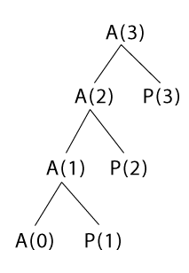
You will first understand the memory representation using trees. It might sound a bit difficult, but it's really straightforward. If you were to write each function call in a tree-like fashion, what would it look like?
Something like the following?

A couple of points to note here:
- The function is called with
A(3)and for that 4 (3+1) function calls are made here. If you generalize this, ifA(n)is called then a total of (n+1) function calls would be required. P()calls are the prints produced byprint(n).- The function stopped with
A(0)function call as theifstatement (afterA(0)function call) will receiven < 1which will cause the function to terminate.
You saw this tree-like representation first because for representing a recursive function on a stack, this representation is needed. You will see that now.
(A stack is a data structure which follows last in first out (LIFO) order of elements)
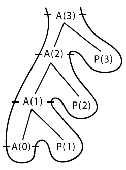
For stack representation, you will have to traverse the tree in a top-down and left-right order. The following image will make this clear.

Interpreting this weird looking thing (tree). Keep in mind that a stack consists of two operations - 1. Push using which you insert an element to the stack & 2. Pop using which you extract an element out of the stack.
Now, you start the tree traversal in a top-down and left-right order:
- Whenever you see a function call, you are going to push that to the stack.
- If you see a
print()/P()call, then you are going to simply print the corresponding element accordingly.
Following is going to be the elements of the stack as a result of the tree traversal from A(3) to A(0) just in the top-down fashion:

Now you start the second half of the tree-traversal, i.e., the left-right order. Whenever you see a function call for the second time you are going to pop it. Surprisingly, the first element of the stack (A(0)) that is going to be popped off from the stack was the last one to enter the stack (LIFO, remember?). Now, in your way you are going to encounter three P() calls - P(1), P(2) and P(3). You are going to print these in the way they arrive in the way of traversal. The order is going to be:
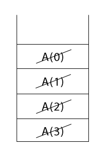
Finally, when you finish the traversal process, the stack will be completely empty. To understand the pop operation even better, here's an image of the stack after being fully popped off.

You saw how to represent a simple recursive function onto memory using a tree and a stack. Now, you will see how to trace a recursion.
Tracing a Recursion:
In this section, you will learn how you can methodically trace a recursion. Consider the following recursive function:
void A(n){
    if(n>0){
        print(n-1);
        A(n-1);
    }
}
One crucial point here is whenever a function is called an activation record is created in the memory which contains the local variables of that function and an instruction pointer (which denotes the next task to be executed when the call returns to that function). Say a function called main() called the above function A() as A(3). Let's number the lines of A() from the if statement for a better understanding:
void A(n){
    1. if(n>0)
    2. {
        3. print(n-1);
        4. A(n-1);
    5. }
}
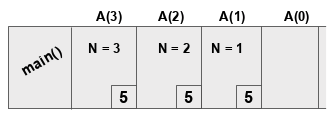
The activation records would look like the following:

As mentioned earlier, the functions have their copies of the local variables and the instruction pointers (in this case the line number). After A(0) the function A() will terminate the popping will take place. Note that, a horizontal stack is used here which is precisely the same as the ones you previously saw in the tutorial. While the records are pushed onto the stack the prints will also take place and the following elements will be printed:
Instruction pointers are vital to note here because often in a recursive function the control goes to the same function but with a different variable value. So, to keep everything in sync these pointers really help. You can follow this exact process in order to trace a recursion using a tree representation.
You will now study how to perform a space-time analysis of a recursive function.
Space-time Analysis of a Recursive Function:
DataCamp has an excellent article on Asymptotic Analysis in Python, and it is recommended that you check it out before reading this section. Let's quickly recap what is meant by space and time analyses of a function (also known as space complexity and time complexity):
For a given input, a function is supposed to produce some kind of output. In order to do that how much time does the function takes? The time-complexity measure approximates this time, and it is also called the runtime of the function. Similarly, the space-complexity measure approximates the space (memory) requirements of a function, i.e., for a given input. But why these are even required?
- Instead of running a function on the range of inputs with varying sizes, you can easily approximate how a function might behave on different inputs with varying sizes.
- If you have two functions that are fulfilling the same objective which one will you take? What measures will you consider to make the decision? Yes, you guessed it right. You will compare them by analyzing their space and time complexities and see which one is performing better.
Let's take a simple recursive function now and analyze its space and time complexity.
void A(n){
    if(n>1) // Anchor condition
    {
       return A(n-1);
    }
}
Let's do the time complexity analysis first. Assume that the total time taken for the above function A() is $T(n)$. Now the $T(n)$ is a sum of the time taken to compare if n is greater than 1 and the time taken to execute A(n-1). So, $T(n)$ can be expressed as -
1 is the time taken for the comparison (you can put any constant there). Now, what will be the time (in terms of $T(n)$) for executing A(n-1)?
Similarly,
and so on.
If you pay close attention to the equations, they all are connected. Aren't they? If you substitute them after one another, you get -
$T(n)$ = 1 + (1 + $T(n-2)$) = 2 + $T(n-2)$ = 3 + $T(n-3)$ = .... = k + $T(n-k)$ (after running the function for k terms)
Now, you need to determine at what point the function is going to stop. According to the anchor condition given, you can write -

Assume that, after running for k terms, the function stops running. If so, then it must be -
$n - k = 1 => k = n - 1$
Now substituting the value of k (= n -1) in $T(n) = k + T(n-k)$ :
$T(n) = (n-1) + T(n-(n-1))$
$=> T(n) = (n-1) + T(1)$
$=> T(n) = n-1 + 1 = n$ // For T(1) only comparison is required
By the rule of asymptotic analysis, $T(n) = n$ can be rewritten as $T(n) = \mathcal{O}(n)$. This means the time complexity (worst) of the function is $\mathcal{O}(n)$.
You might want to slow down a bit here and observe each step of this process carefully. It's highly recommended that you do this on a pen and paper so that you can understand every bit of it.
The space complexity analysis of the function is simple. The function is an in-memory function and does not make use of any extra variables. So, you can conclude that the space complexity of the function $\mathcal{O}(n)$.
Now you will put all these together and implement a simple recursive function in Python.
Implementing a Simple Recursive Function in Python:
You will write a recursive function to find the factorial of a given number. You will then write an iterative version of the same function. Let's get started.
# Recursive function factorial_recursion()

def factorial_recursion(n):
   if n == 1:
       return n
   else:
       return n*factorial_recursion(n-1)
# Call the function

num = 7
print("The factorial of ",num," is ",factorial_recursion(num))
The factorial of 7 is 5040
Remember the two key ingredients for writing a recursive function?
- Recurrence relation
- Termination condition
In this case, the recurrence relation can be -
$f(n) = n!$
$f(n) = n * f(n-1)$ and so on.
The termination condition is when n is equal to 1.
Simple, right?
Now, you will implement the iterative version of the same function.
def factorial_iterative(num):
    factorial = 1
    if num < 0:
        print("Sorry, factorial does not exist for negative numbers")
    elif num == 0:
        print("The factorial of 0 is 1")
    else:
        for i in range(1,num + 1):
           factorial = factorial*i
        print("The factorial of",num,"is",factorial)
factorial_iterative(7)
The factorial of 7 is 5040
You can clearly spot the difference between the two versions. The recursive version is way more beautiful than the iterative version. Isn't it?
Congrats!
You have made it till the end. In this tutorial, you did an extensive study of recursive functions. Starting from the absolute basics to analyzing the space and time complexities of a recursive function, you covered it all. You also saw, how recursion can be beneficial for solving problems with a particular characteristic. Now, you should be in a position to solve problems (having a recurrence relation and a termination condition) using recursion. You might want to solve the problem of finding Fibonacci Numbers within a range using recursion.
I will insist you to solve some common problems like Binary Search, Merge Sort, Tower of Hanoi, etc. using recursion and perform a space-time analysis as well. This will certainly make you a better programmer.
From an introductory aspect, the things you covered are sufficient. But if you want to study more about recursion, make sure you visit the following links:
- Recursion and Dictionaries by Prof. Grimson
- Dynamic Programming to optimize the performance of recursive functions
If you want to learn more about Python, take DataCamp's free Intro to Python for Data Science course.