Excel IFERROR(): How to Handle Errors in Excel Formulas

In this article, I’ll show you how the IFERROR() function can help you clean up some common and annoying errors such as the #DIV/0! or #N/A error. Personally, I don’t like seeing these errors messages in my workbooks, so I expect that you probably don’t like seeing these errors, either. Together, we will work through how to solve all this.

After we are done solving this particular issue, I recommend, if you find yourself running into other kinds of trouble, that you take our Excel Fundamentals skill track to grow your skills.

What Is the Excel IFERROR() Function?

The Excel IFERROR() function allows you to catch and handle errors in your formulas. Instead of displaying error messages like #DIV/0! or #N/A, IFERROR() lets you show a custom result or message. This helps keep your spreadsheets looking clean. Plus, it makes them easier to understand.

Excel IFERROR() Syntax

The  IFERROR() function requires two arguments:

IFERROR(value, value_if_error)

• value: The formula or expression you want to check for errors.

• value_if_error: The value to return if an error is found.

How to Use Excel IFERROR() in Formulas

You can use IFERROR() with any formula that might return an error. Here’s how to apply it:

=IFERROR(A1/B1, "Don't forget that you can't divide by zero!")

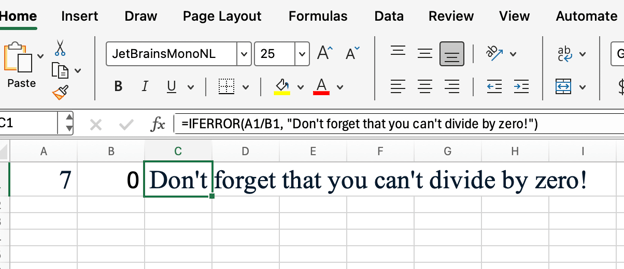
If B1 is zero, Excel would normally display #DIV/0!. With IFERROR(), it will show "Don't forget that you can't divide by zero!" (or whatever other message you want to say) instead.

Common Uses for Excel IFERROR()

There are several scenarios where IFERROR() is especially useful. Here are some common examples:

• Handling division by zero errors (I chose this as the main example for a reason.)

• Managing lookup errors with VLOOKUP() or MATCH()

• Replacing #N/A or #VALUE! errors with custom messages

Using Excel IFERROR() with Other Functions

You can combine IFERROR() with other Excel functions to improve your formulas. I mentioned VLOOKUP(), so let me show that now:

=IFERROR(VLOOKUP(A1:A3, B1, 1, FALSE), "Not found")

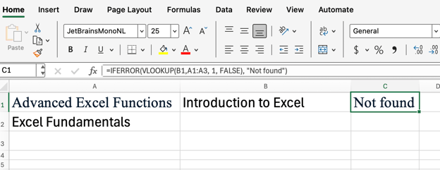
If VLOOKUP() cannot find a match, the formula will return "Not found" instead of #N/A.

Tips for Using Excel IFERROR() Effectively

To get the most out of IFERROR(), keep these tips in mind:

• Use clear, descriptive custom messages
• Avoid hiding errors that need attention
• Combine with other error-checking functions for stronger overall formulas

Excel IFERROR() vs. ISERROR() and IFNA()

It’s important to understand how IFERROR() compares to similar functions. Here are two similar-sounding ones that come to mind:

• ISERROR(): Returns TRUE if a value is any error, but requires a separate IF() statement to handle errors.

• IFNA(): Only catches #N/A errors, not other types.

I think IFERROR() is generally more versatile for most cases that you're going to run into.

Conclusion

By using IFERROR(), you can create cleaner, more user-friendly spreadsheets and prevent confusing error messages from appearing. Experiment with IFERROR() in your own workbooks to see how it can improve your Excel experience. And while you're practicing, take our Advanced Excel Functions course to keep getting better and faster with Excel.