Logistic Regression Assumptions: What You Need to Check Before Modeling

After you’ve trained a logistic regression model, how can you be sure you can trust the coefficients?

Logistic regression is known for being simple. With scikit-learn, you call .fit(), read off the odds ratios, and that’s about it. But what most beginners don’t know is that the model has its own assumptions, and when you don’t follow them, the coefficients mislead you and the predictions are off in ways no test metric will tell you.

Truth be told, logistic regression has fewer assumptions than linear regression, and the ones it does have are easy to check. You just need to run the right diagnostics before interpreting the output to know which parts of the model to trust.

In this article, I'll walk you through every assumption logistic regression makes, how to check each one in Python and R, what happens when they're violated, and which alternatives to reach for when the assumptions can’t be followed.

If you’re new to data science and machine learning, read our blog post on Simple Linear Regression to understand its assumptions and diagnostics.

What Is Logistic Regression?

Logistic regression is a classification model that predicts the probability of a categorical outcome. You give it predictors, and it returns a number between 0 and 1 that you can read as the probability of belonging to a given class.

Most people use it for binary classification like churn or no churn, spam or not spam. Variants like multinomial and ordinal logistic regression cover more than two classes, but the binary case is what most people mean when they say "logistic regression."

Below the surface, the model fits a linear combination of your predictors and passes the result through the logistic function. The output is a probability, and the coefficients tell you how each predictor shifts the log-odds.

It’s worth noting that logistic regression is different from linear regression. The prior has familiar assumptions such as normality of residuals, homoscedasticity, linearity between predictors and target. Logistic regression doesn't make those assumptions. It has its own list, and they're different enough that using assumptions of a linear regression will give you misleading results.

For more details on logistic regression, read our blog post that shows implementation in Python.

Why Logistic Regression Assumptions Matter

The assumptions matter because they directly connect to what you do with the model.

If you respect the assumptions, the coefficients mean what you think they mean. The odds ratios you read are valid, and the model's probabilities map well to actual outcomes. When the assumptions aren’t respected, all of that gets shaky in ways a confusion matrix or any other metric won’t show you.

The good thing is that violations aren't binary. A mild deviation from, say, the linearity-of-the-logit assumption won't make your model useless. It just means your odds ratios are slightly off and your predictions could be worse than they should be. Plenty of production models live with imperfect assumption checks, and that's fine.

What you don't want is to skip the checks. Without diagnostics, you can't tell if you're looking at a small or a big problem until predictions go wrong.

Overview of Logistic Regression Assumptions

Before getting into each assumption, here's the full list you'll need to check.

Logistic regression assumptions table

That's the whole checklist. In the rest of the article, I’ll walk you through each assumption with diagnostics in Python and R, what a violation looks like, and what to do when something goes wrong.

The Main Logistic Regression Assumptions

Assumption 1: The outcome variable is binary (or appropriately modeled)

Standard logistic regression is built for a binary outcome. The target variable should have exactly two categories, and the model is designed around that case.

The classic examples are churn or no churn, disease or no disease. Anything you can phrase as a yes/no question is a good fit.

When your outcome has more than two categories, you need a different variant. Multinomial logistic regression handles unordered categories like customer segments or product types. Ordinal logistic regression handles ordered categories like satisfaction scores from 1 to 5, where the order between levels has meaning.

Forcing a multi-class outcome into a binary model usually means collapsing categories you shouldn't collapse. If you have a satisfaction target with five levels and you cut it down to "satisfied vs not," you lose information that could have helped your model. Pick the variant that matches the shape of your target.

Assumption 2: Observations are independent

Each row in your dataset should give the model information no other row already provides. If two records are linked in a way that violates this, your standard errors and p-values won't mean what they should.

The assumption fails any time observations share structure you haven't modeled. A good example is repeated measurements on the same patient, as it shares that patient's biology. Another example is students grouped within the same classroom, as they share the teacher and the room.

When you ignore this and fit a plain logistic regression, the model treats each row as new information and reduces the standard errors more than it should. Coefficients can still look fine on the surface, but the p-values and confidence intervals will be overconfident.

The standard alternatives are mixed-effects logistic regression and GEE. Mixed-effects models add random effects for the groups (patient, classroom) so the model accounts for within-group correlation. GEE, short for generalized estimating equations, gives you population-averaged effects with corrected standard errors, without the random-effects machinery.

Pick mixed-effects when you care about within-group variation. Pick GEE when you want marginal effects across the whole population.

Assumption 3: Linearity of the logit

This is the assumption most people get wrong about logistic regression.

The model does not assume your predictors have a linear relationship with the outcome. It assumes they have a linear relationship with the log-odds of the outcome. That's a different statement, and it changes what you should check.

What the logit is

The logit is the natural logarithm of the odds. For a probability p, the odds are p / (1 - p), and the logit is the log of that ratio:

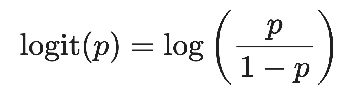
The logit

Logistic regression then fits a linear equation on this scale:

Logistic regression formula

The right-hand side is linear in the predictors. The left-hand side is the log-odds, not the probability. The probability you actually care about is recovered by passing the linear combination through the logistic function, which is nonlinear.

So the relationship between any predictor and the probability is nonlinear. The relationship between any predictor and the log-odds is what should be linear.

Why this matters in practice

When the linearity of the logit doesn't hold for some predictor, the coefficient on that predictor is summarizing a curve with a straight line. The model still gives you a number, and the number can still be statistically significant, but the number doesn't describe the actual relationship in your data.

For example, age might have a U-shaped effect on the log-odds of a disease, with high risk at both ends and lower risk in the middle. If you stick age in as a single linear term, the coefficient might come out close to zero and you'll conclude age doesn't matter. It does. The specification is wrong.

Checking the linearity of the logit

You have a few options for checking this assumption.

The fastest check is visual inspection. Bin each continuous predictor into deciles, compute the empirical log-odds within each bin, and plot the result against the predictor. A roughly straight line means the assumption holds. A clear curve means it doesn't. The check is informal but works well when you have enough data per bin.

The Box-Tidwell test adds an interaction term between each continuous predictor and its own natural log. If the interaction is statistically significant, the linearity-of-the-logit assumption is violated for that predictor. The test only works on strictly positive predictors (since you can't take the log of zero or a negative number), and it's sensitive to sample size like any significance test.

Splines are another option. Instead of checking whether linearity holds, you replace the linear term with a flexible basis function like a restricted cubic spline, and let the model fit the shape it needs. If the spline fits much better than the linear term (judged by likelihood ratio or AIC), you have evidence the linear specification was too restrictive. Splines also double as a fix. Keeping them in the final model is often the best answer when linearity fails.

What to do when linearity fails

If the assumption fails for a predictor, you have a couple of options:

• Transform the predictor (a log or square-root transform often does it) until the relationship looks linear in the log-odds
• Use splines and accept a slightly more complex model

Both keep you in the logistic regression family, and both are better than excluding a predictor that's actually informative.

Assumption 4: No severe multicollinearity

Logistic regression handles correlated predictors up to a point. After that point, the model starts to misbehave in ways that are hard to spot from any test metric.

Multicollinearity happens when two or more predictors have the same (or really similar) information. Maybe you have height in inches and height in centimeters in the same model. Maybe you have total revenue and revenue per customer alongside customer count.

Two things go wrong when multicollinearity is present:

• Coefficients become unstable: If you add or drop a single row, the coefficient on a collinear predictor can swing or flip sign. The model still works, but the individual coefficients are not meaningful.
• Standard errors inflate: With less independent information per predictor, the model becomes less certain about each coefficient. P-values rise, and real effects can come back as not significant.

Predictions are usually fine. If you only care about the predicted probability, mild to moderate multicollinearity rarely causes problems. The “damage” is concentrated in the coefficients and the inference you do on them.

The two checks are a correlation matrix and the variance inflation factor (VIF). A correlation matrix is the first thing to look at, especially pairs of predictors with correlations above 0.8 or 0.9 in absolute value. The limitation is that correlation matrices only catch pairwise collinearity, not the multi-way case where three or more predictors are collectively redundant.

VIF is here for the multi-way case. For each predictor, VIF measures how much the variance of its coefficient is inflated by collinearity with the rest of the predictors. A VIF of 1 means no collinearity, values up to 5 are usually fine, and values above 10 are a strong signal that the predictor is redundant with others in the model.

When VIF flags something, the easiest fix is to drop one of the collinear predictors or combine them into a single feature like a sum or a ratio. If you'd rather keep all predictors, regularization (ridge or elastic net) stabilizes the coefficients without making you choose.

Assumption 5: Adequate sample size

Logistic regression works with small samples, but is somewhat unreliable. Coefficients swing more than they should, and rare-class effects become nearly impossible to estimate.

The sample size that matters for logistic regression isn't the total row count. It's the number of events (observations in the minority class). A dataset with 100,000 rows and 50 fraud cases is a small-sample problem, because the model only has 50 examples of the thing it's trying to learn.

That's where events per variable (EPV) comes in. EPV is the number of minority-class observations divided by the number of predictors in the model. If you have 50 fraud cases and 10 predictors, your EPV is 5.

The old rule of thumb was an EPV of at least 10. More recent simulation work has shown that the right number depends on the effect sizes in your data and the amount of regularization you're using. EPVs as low as 5 can be fine in some settings, and EPVs of 20 or more may be needed in others.

The takeaway is to treat EPV as a warning information. Below 10, expect unstable estimates and consider penalized methods like Firth's logistic regression or ridge. Below 5, get more data or simplify the model before trusting any individual coefficient.

Class imbalance is a related but distinct problem.

A dataset where 99% of cases are one class can still have plenty of events per variable in absolute terms. What shifts is the base rate of the outcome, not the EPV. Imbalanced data tends to produce conservative probability estimates, and accuracy stops being a useful metric. To get around it, evaluate with log-loss or Brier score instead of accuracy, and consider class weights or threshold tuning if you need balanced decisions.

Assumption 6: No highly influential outliers

Logistic regression doesn't assume your predictors are normally distributed. Skewed predictors and count variables are all fine on their own. What the model does care about is if any single observation has outsized influence on the fitted coefficients.

An influential observation is one that, if you removed it, would meaningfully change the model. It's not the same as a residual outlier. A point can have a large residual (the model predicts it badly) without being influential, and a point can be highly influential (the model leans heavily on it) without having a large residual.

You'll want a few diagnostics that look at different aspects of influence:

• Leverage measures how unusual an observation's predictor values are relative to the rest of the data. Leverage alone doesn't mean an observation is influential. It means the point has the potential to be influential if its outcome doesn't match what its predictors would suggest
• Cook's distance combines leverage with the residual into a single number that estimates how much the fitted coefficients would change if you dropped the observation. Large Cook's distance values highlight the points worth investigating. Common conventions are values above 4/n (where n is your sample size) or just looking at the largest couple of Cook's distance values in your dataset
• Residual diagnostics are great for the cases leverage and Cook's distance don't catch. Deviance residuals and Pearson residuals flag observations the model has trouble fitting. A point with a large residual is worth a look even if its leverage is moderate, since the model is telling you it can't explain that case with the other predictors

When you find an influential point, the question is whether the point is real or wrong. A data-entry error gets fixed or removed. A real but unusual case stays, and you note that your conclusions depend on it. Just don't exclude points because they're influential. That's how you end up with a model that fits your training data and nothing else.

Common Misconceptions About Logistic Regression Assumptions

Most of the confusion around logistic regression's assumptions comes from using linear regression's checklist. Linear regression's assumptions are well-known and taught everywhere, and they show up in logistic regression where they don't belong. Here are the four most common ones to clear up.

Logistic regression requires normally distributed variables

This is false. Logistic regression makes no normality assumption on any variable in the model.

The outcome is supposed to be binary, not normal, and we've covered that in Assumption 1. The predictors aren't assumed normal either, and they can take whatever shape the data has. What matters is the relationship between the predictors and the log-odds, not the marginal distribution of any single variable.

Logistic regression requires homoscedasticity

This is false too. Homoscedasticity (constant variance of residuals across the range of predicted values) is a linear regression assumption that doesn't apply to logistic regression.

The variance of the outcome in logistic regression depends on the predicted probability itself. For a Bernoulli outcome, variance equals p(1 - p), which is highest near p = 0.5 and lowest near 0 and 1. The variance isn't constant, and the model accounts for that through the likelihood function it maximizes.

So when you fit a logistic regression, you're not violating anything by having predicted probabilities with different variances. That's just how the model works.

Predictors must be normally distributed

This is false. Logistic regression places no distributional assumption on the predictors.

You can mix continuous, binary, count, and categorical predictors in the same model. Skewed predictors are fine. Heavy-tailed predictors are fine. The model doesn't care about marginal shapes. The only thing it does care about is the linearity of the logit (covered in Assumption 3), which is a relationship-shape assumption, not a distribution-shape assumption.

If a predictor's skew creates problems, it's usually because of the linearity of the logit or influential outliers.

Residuals must be normally distributed

This is false. There's no normality assumption on logistic regression's residuals.

Linear regression assumes that residuals are normally distributed around zero, because that's part of how its inference works. Logistic regression uses maximum likelihood estimation on a binomial likelihood, and the distribution of its residuals is determined by the outcome (which is 0 or 1) and the fitted probability. They aren't normal, and they aren't supposed to be.

So when you check residual diagnostics for logistic regression (as in Assumption 6), you're looking for influential observations and points the model can't explain, not for a bell curve.

How to Check Logistic Regression Assumptions in Python

I’ll do the diagnostics with statsmodels. Scikit-learn fits logistic regression but doesn't give you VIF, influence statistics, or residual diagnostics out of the box.

Setting up the example

I'll generate a synthetic churn dataset with three predictors (age, income, and spending score), where age and income are deliberately correlated so multicollinearity has something to find.

import numpy as np
import pandas as pd
import statsmodels.api as sm
import statsmodels.formula.api as smf

np.random.seed(42)
n = 1000

age = np.random.normal(40, 12, n).clip(18, 80)
income = 30000 + 1500 * age + np.random.normal(0, 8000, n)
spending_score = np.random.uniform(1, 100, n)
logit_p = -3 + 0.04 * age + 0.02 * spending_score
p = 1 / (1 + np.exp(-logit_p))
y = np.random.binomial(1, p)

df = pd.DataFrame({
    "churned": y,
    "age": age,
    "income": income,
    "spending_score": spending_score,
})

model = smf.glm(
    "churned ~ age + income + spending_score",
    data=df, family=sm.families.Binomial()
).fit()
print(model.summary())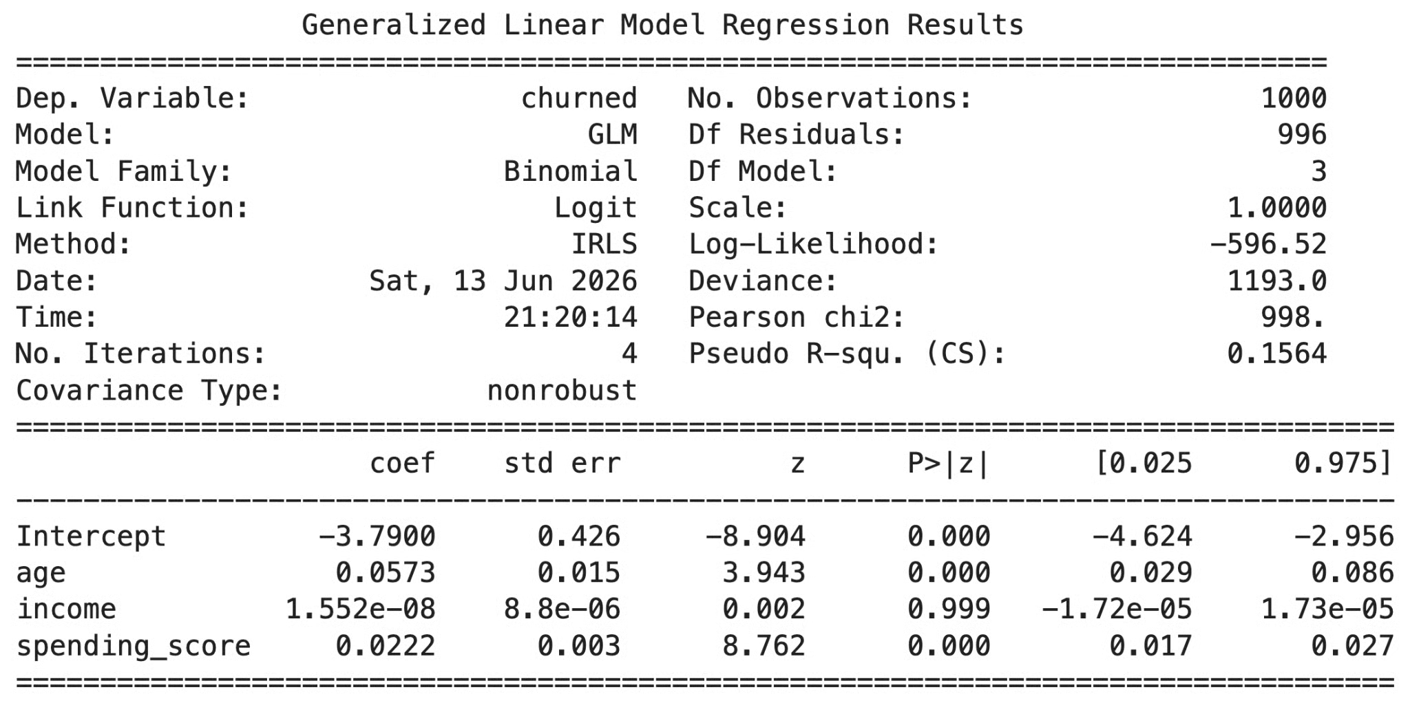

Model summary

The summary gives you coefficients, standard errors, z-statistics, and p-values. age and spending_score come out as the meaningful predictors. The coefficient of income is tiny because the outcome doesn't directly depend on income. Its apparent effect gets absorbed by age.

Multicollinearity with VIF

Statsmodels makes this computation incredibly easy:

from statsmodels.stats.outliers_influence import variance_inflation_factor

X = sm.add_constant(df[["age", "income", "spending_score"]])
vif = pd.DataFrame({
    "feature": X.columns,
    "VIF": [variance_inflation_factor(X.values, i) for i in range(X.shape[1])]
})
print(vif[vif["feature"] != "const"])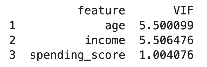

VIF output

The VIFs for age and income come out around 5.5, which shows mild multicollinearity. spending_score comes out near 1, which is what you want. Its variance isn't being inflated by collinearity with the others. VIFs above 5 are mild flags; above 10 are a serious problem you need to resolve immediately. The move here is to either drop one of age or income or combine them into a single feature.

Linearity of the logit with Box-Tidwell

The Box-Tidwell test adds interaction terms between each continuous predictor and its own natural log. Significant interactions flag a non-linear log-odds relationship for that predictor.

df_bt = df.copy()
for col in ["age", "income", "spending_score"]:
    df_bt[f"{col}_logx"] = df_bt[col] * np.log(df_bt[col])

bt_formula = (
    "churned ~ age + income + spending_score + "
    "age_logx + income_logx + spending_score_logx"
)
bt_model = smf.glm(
    bt_formula, data=df_bt, family=sm.families.Binomial()
).fit()

interactions = ["age_logx", "income_logx", "spending_score_logx"]
print(bt_model.pvalues[interactions])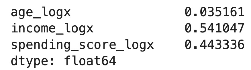

Box-Tidwell output

If any of these p-values come out below 0.05, the linearity-of-the-logit assumption is suspect for that predictor. The logit was generated linearly here, so the interactions shouldn't be significant. On real data, treat a significant result as a prompt to plot the empirical log-odds against that predictor and decide whether a transformation or a spline is the right fix.

Influence diagnostics

Statsmodels gives you access to Cook's distance and leverage through get_influence().

influence = model.get_influence()
cooks_d = influence.cooks_distance[0]
leverage = influence.hat_matrix_diag

flagged = pd.DataFrame({
    "cooks_d": cooks_d,
    "leverage": leverage,
}).sort_values("cooks_d", ascending=False).head(10)
print(flagged)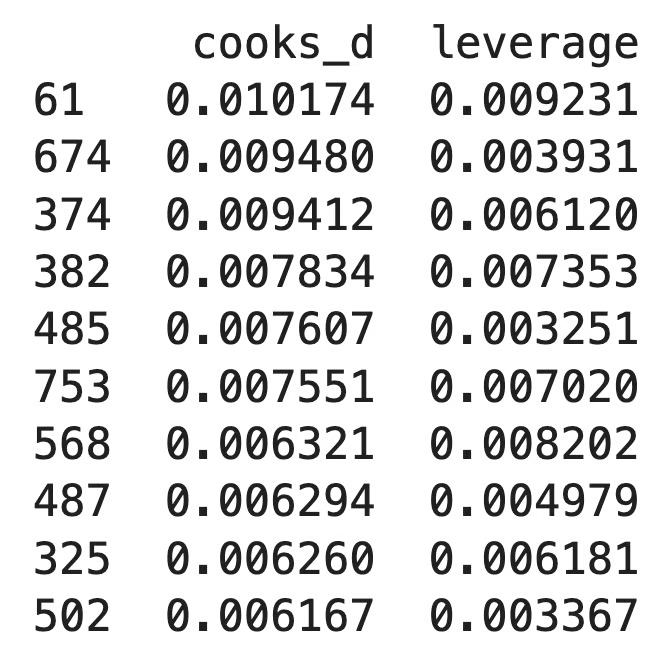

Influence diagnostics output

The threshold for Cook's distance worth investigating is roughly 4/n. With 1000 rows, that's 0.004. Anything well above that needs a closer look. In this dataset, the largest Cook's distances are still small in absolute terms, which is the boring-good outcome you usually want.

Let me now create a visualization to make the distribution easier to read:

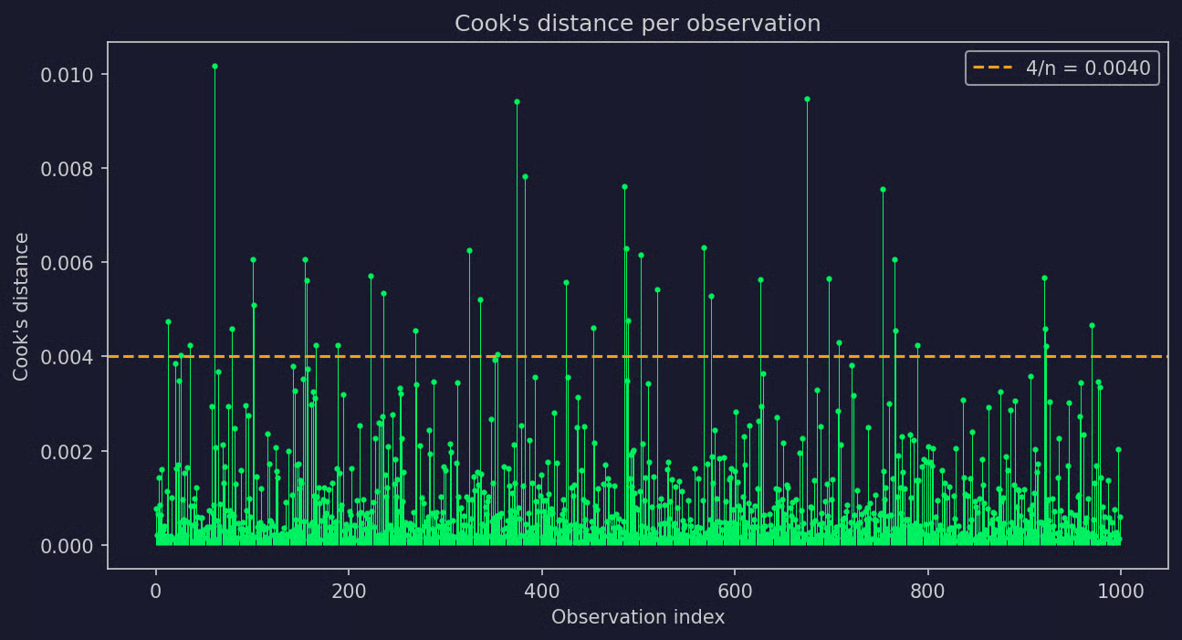
Influence diagnostics visualized

Points sitting well above the dashed threshold are the ones to investigate. There are some, but not too many.

Residual diagnostics

The deviance residuals tell you which observations the model is having trouble fitting.

deviance_resid = model.resid_deviance
fitted = model.fittedvalues

resid_df = pd.DataFrame({
    "fitted": fitted,
    "deviance": deviance_resid,
}).sort_values("deviance", key=abs, ascending=False).head(10)
print(resid_df)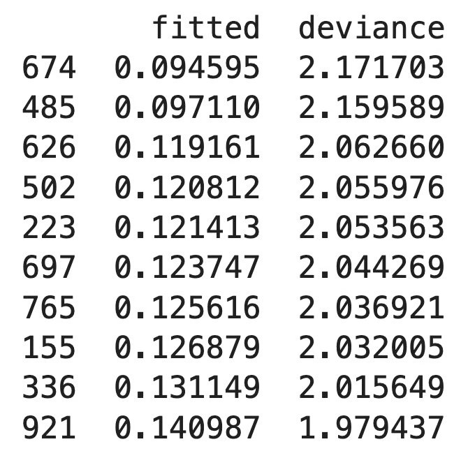

Residual diagnostics output

Large positive deviance residuals are cases where the model assigned a low probability but were actually positive. Large negative residuals are the reverse. You should cross-reference high-residual observations with the influence diagnostics above. A case that's both badly predicted and influential is the one most worth investigating.

How to Check Logistic Regression Assumptions in R

R has tighter built-in support for these diagnostics. Most of what you need comes from base R's glm() plus the car package.

Setting up the example

I'll generate the same kind of synthetic dataset as the Python example, with age and income deliberately correlated.

set.seed(42)
n <- 1000

age <- pmin(pmax(rnorm(n, mean = 40, sd = 12), 18), 80)
income <- 30000 + 1500 * age + rnorm(n, sd = 8000)
spending_score <- runif(n, min = 1, max = 100)
logit_p <- -3 + 0.04 * age + 0.02 * spending_score
p <- 1 / (1 + exp(-logit_p))
churned <- rbinom(n, size = 1, prob = p)

df <- data.frame(churned, age, income, spending_score)

model <- glm(churned ~ age + income + spending_score,
             data = df, family = binomial)
summary(model)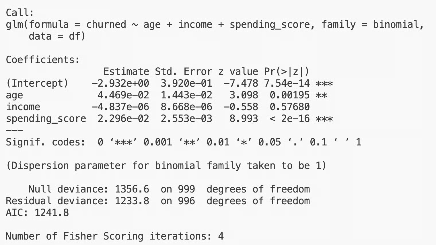

Model summary output

The summary(model) output gives you coefficients, standard errors, z-statistics, and p-values. age and spending_score should look meaningful, while the effect of income gets absorbed by age.

Multicollinearity with VIF

The car package gives you vif() for any glm:

library(car)

vif(model)

VIF output in R

age and income will both come back with VIFs around 5.7, which shows the multicollinearity built into the data. spending_score is near 1. As in Python, values above 5 deserve attention and values above 10 are a clear problem.

Linearity of the logit with Box-Tidwell

The car::boxTidwell function is designed for linear regression, so for logistic regression the best approach is to add the interaction terms manually and refit:

df_bt <- df
df_bt$age_logx <- df_bt$age * log(df_bt$age)
df_bt$income_logx <- df_bt$income * log(df_bt$income)
df_bt$spending_score_logx <- df_bt$spending_score * log(df_bt$spending_score)

bt_model <- glm(
  churned ~ age + income + spending_score +
    age_logx + income_logx + spending_score_logx,
  data = df_bt, family = binomial
)

interactions <- c("age_logx", "income_logx", "spending_score_logx")
summary(bt_model)$coefficients[interactions, ]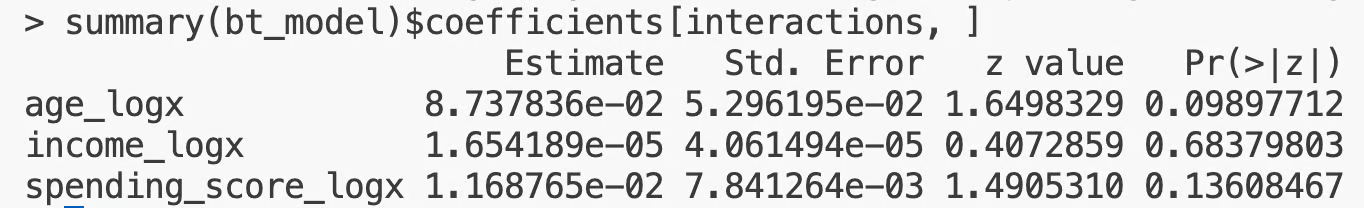

BoX-Tidwell output in R

The output shows the coefficient and p-value for each interaction term. Significant p-values flag a violation of the linearity-of-the-logit assumption for that predictor. For the synthetic data here, the test shouldn't reject linearity. On real data, follow up with empirical log-odds plots or fit a model with splines (from the splines package) for any predictor the test flags.

Influence diagnostics

R provides cooks.distance() and hatvalues() in base, so no third-party package is needed:

cooks_d <- cooks.distance(model)
leverage <- hatvalues(model)

influence_df <- data.frame(
  index = seq_along(cooks_d),
  cooks_d = cooks_d,
  leverage = leverage
)
head(influence_df[order(-influence_df$cooks_d), ], 10)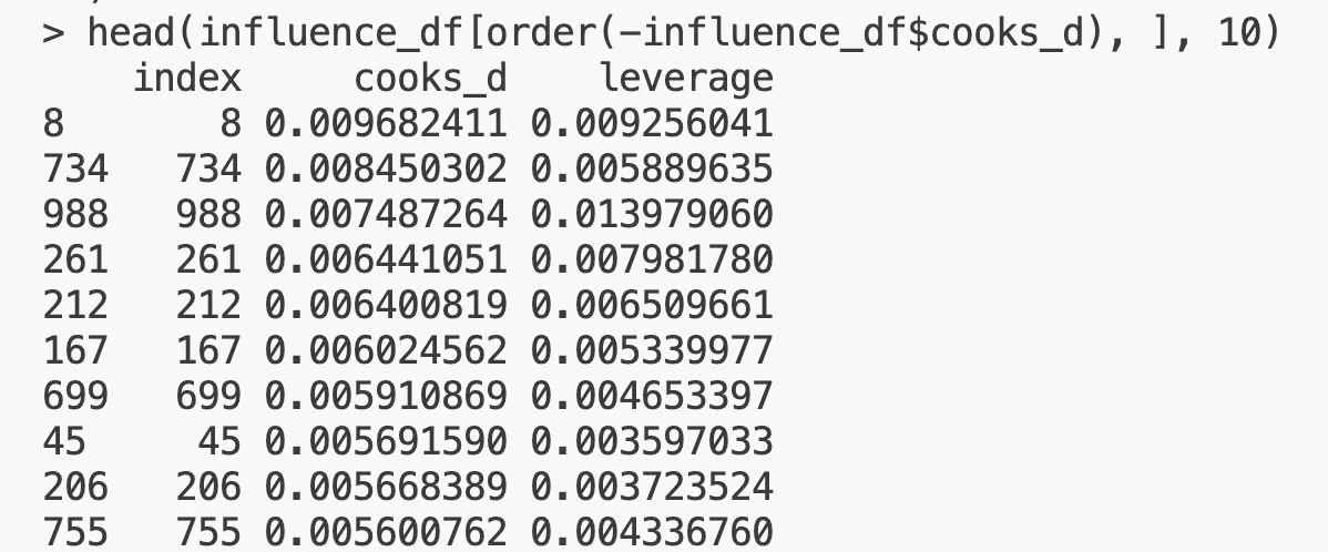

Influence diagnostics in R

The threshold for Cook's distance is the same as in Python: 4/n, or 0.004 for the 1000-row dataset. Anything well above that deserves investigation. For a quick visual check, base R's plot(model, which = 4) gives a Cook's distance plot in one line.

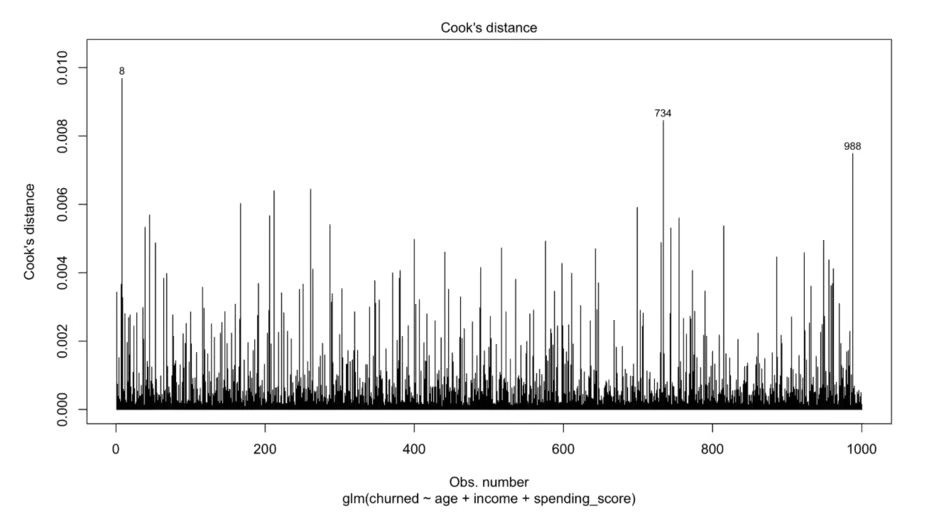
Influence diagnostics in R visualized

Residual diagnostics

R's residuals() function gives you deviance residuals from a glm:

deviance_resid <- residuals(model, type = "deviance")
fitted_vals <- fitted(model)

resid_df <- data.frame(
  fitted = fitted_vals,
  deviance = deviance_resid
)
head(resid_df[order(-abs(resid_df$deviance)), ], 10)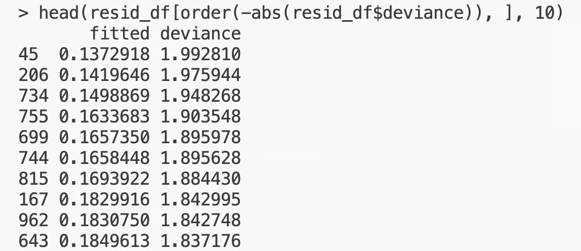

Residual diagnostics in R

Large absolute deviance residuals are cases the model's prediction missed. You should cross-reference these with the Cook's distance flags above to find observations that are both poorly fit and influential.

For a one-shot view of everything, influence.measures(model) returns a table that combines Cook's distance, leverage, DFBETAs, and a couple of other influence statistics in one place. It's the fastest way to scan all the standard diagnostics on a fitted glm.

What Happens When Assumptions Are Violated?

Most assumption violations won’t break your model in the way that it doesn’t work. They cause it to misbehave in subtle ways that you only notice if you know what to look for.

Four consequences come up most of the time:

1. Unstable coefficients: Small changes in the data (a few rows added or dropped, a slight change to feature engineering) can drastically change the coefficients or flip their signs. This is what multicollinearity does, and it's also what happens when your sample size is too small for the number of predictors
2. Poor calibration: The model's predicted probabilities stop matching the actual rates in the data. It predicts 30% churn for a group and observe 15%. Accuracy might still look fine, but the probabilities are off. Violations of linearity in the logit and influential outliers both contribute to this
3. Misleading inference: This one is the hardest to spot, because the model still produces standard errors and p-values that look fine. Correlated observations reduce standard errors below where they should be, and the wrong predictor specifications inflate them. Either way, the p-values you get don't mean what you think they mean
4. Degraded prediction quality: The most obvious symptom, even though it's often the smallest in practice. Predictions usually hold up better than the coefficients do, which is why teams that focus only on accuracy often miss the warning signs.

But honestly, violations rarely make a model useless. They make parts of it unreliable, and the parts that are unreliable depend on which assumption broke. That's why the diagnostics matter.

Alternatives When Logistic Regression Assumptions Fail

If your diagnostics point to problems you can't fix within logistic regression, the next move is to use a model that doesn't make those assumptions.

Generalized additive models (GAMs) are the next thing to look for. A GAM keeps the logistic link function and the interpretable additive structure, but replaces the linear terms with smooth functions of each predictor. You get coefficients-with-shapes instead of single numbers, which solves the linearity-of-the-logit problem. GAMs are still parametric enough to inspect and interpret, which makes them a good step up from logistic regression when the linearity assumption can’t hold.

Tree-based models are the more flexible alternative. Random forests and gradient boosting make no assumptions about predictor distributions or relationship shapes. They handle multicollinearity and can even capture nonlinearity. They don’t give you the easy coefficient interpretation that logistic regression offers, but they tend to outperform on predictive metrics when the data has nonlinear structure or interactions you didn't put in the model.

The choice between GAMs and tree-based models comes down to what you need from the model.

• Pick GAMs when interpretability is the priority and you want to see how each predictor affects the log-odds
• Pick a gradient-boosted tree when prediction quality is the priority and you can accept a less transparent model

It’s worth noting that logistic regression's assumptions are easier to check than to ignore. If you can fix the issue with a transformation, a spline, regularization, or a better sample, logistic regression's interpretability and inferential output usually beat what you get from a switch to a more flexible model.

So, move to GAMs or trees when the diagnostics tell you the assumptions really don't hold, not just because logistic regression isn't a state of the art algorithm.

Best Practices for Logistic Regression Modeling

And finally, follow this short list to always get a model you can trust:

• Inspect assumptions before interpretation: Run VIF, the Box-Tidwell test, and influence diagnostics before you read off the coefficients. If you interpret first and check later, you'll find yourself defending numbers you didn't verify. You don’t want to be that person in a meeting
• Use regularization when sample size is small: Ridge or elastic net stabilizes coefficients when EPV is low or predictors are correlated. The trade-off is a small bias for a large variance reduction, which is usually a good deal
• Validate on data the model hasn't seen: Hold out a test set or use cross-validation. Training metrics overstate performance whenever the model has room to overfit, which logistic regression does whenever you have many predictors or rare events
• Evaluate calibration: Accuracy hides whether your predicted probabilities map to actual rates. Use log-loss or Brier score for evaluation, and look at a calibration plot when probabilities matter for business decisions

Conclusion

Truth be told, logistic regression is one of the more forgiving models you can fit.

It tolerates skewed predictors and imbalanced outcomes, and it doesn't care what your residuals look like. What it can't tolerate is a misspecified relationship with the log-odds, or a set of predictors that all have the same information.

That's why linearity of the logit and multicollinearity are the two assumption checks worth treating as required. They're the ones that distort the model in ways no test metric can catch. Other four assumptions are also relevant, but these two are what you should really focus on.

To be safe, run the diagnostics alongside the evaluation, not after it. A model that predicts well and passes its assumption checks is a model you can stand behind. Anything less is a model you've trained but haven't really verified.

If this sounds complex, it’s because it is. It takes a lot to be a good machine learning engineer, so we recommend you to enroll in our Machine Learning Scientist in Python track. 85 hours of materials will get you job-ready for 2026.