Curso
Data science is an interdisciplinary field that uses mathematics and advanced statistics to make predictions. All data science algorithms directly or indirectly use mathematical concepts. Solid understanding of math will help you develop innovative data science solutions such as a recommender system. If you are good at mathematics, it will make your transition into data science easier. As a data scientist, you have to utilize the fundamental concepts of mathematics to solve problems.
Apart from mathematics, you also need domain knowledge, programming skills, business skills, analytical skills, and a curious mindset. There is no way of escaping mathematics for a data scientist. You have to inculcate and teach yourself the basics of mathematics and statistics to become a data scientist.
Scalar and Vector
- Scalars: A scalar is a single number that deals with the vector in space via scalar multiplication.
- Vectors: A vector V is an ordered set of items. Vector is an array of numbers that can be a row or a column. Vectors can be added together and can be multiplied by a real number known as a scaler.

# Import numpy module
import numpy as np

# creating a vector
v = np.array([1, 2, 3, 4, 5])
print(v)
[1 2 3 4 5]
# Vector Operations
# Import numpy module
import numpy as np

# Create two vector
a = np.array([1, 2, 3, 4, 5])
b = np.array([1, 2, 3, 4, 5])

# adding two vectors
add = a + b
print("Addition:",add)

# Vector Subtraction
sub = a - b
print("Subtraction:",sub)

# Vector Multiplication
mul = a * b
print("Multiplication:",mul)

# Vector Division
div = a / b
print("division",div)
Addition: [ 2  4  6  8 10]
Subtraction: [0 0 0 0 0]
Multiplication: [ 1  4  9 16 25]
division [1. 1. 1. 1. 1.]
Matrix and Tensor
- Matrices: A matrix is an N-D array of numbers which represent transformations. You can think of a matrix as a transformation such as "scale", "rotate", "shear", and "flip". It turns single points in space into different points in space.
# Import numpy module
import numpy as np

# create 2*2 matrix
a1=np.array([[1, 2], [3, 4]])
a2=np.array([[1, 2], [3, 4]])

# Dot Product
dot_product = np.dot(a1,a2)
print("Dot Product: \n",dot_product)

# Cross Product
cross_product = np.cross(a1,a2)
print("Cross Product: \n", cross_product)
Dot Product:
 [[ 7 10]
 [15 22]]
Cross Product:
 [0 0]
Dot Product of two vectors represents the projection of one vector on another vector and Cross Product of two vectors enables one vector to identify the plane on which both the vectors can lie.
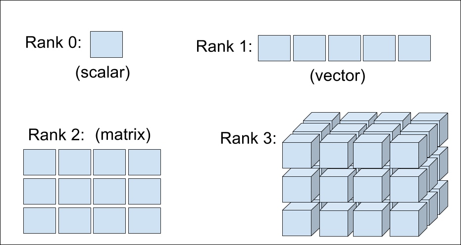
- Tensor: Sometimes, you will need an array with more than two dimensions and with a different dimension of each array, arranged in a grid known as a tensor. Tensor dimension is known as its rank. Scalars and vectors are also a type of tensor. Zero-order tensors are scalers, and first-order tensors are vectors.
Determinant
Determinant is a scalar value that represents a factor of a matrix by which length(in 1-dimension), area(2-dimension), volume (3-dimension) can be explored. If the determinant is 2, it is twice the volume(in 3-dimension), or if the determinant is 1, it will not affect the volume(in 3-dimension). If the determinant is 0, it has no inverse because zero multiplied with anything will give you zero.

Properties:
-
The product of matrices is the product of the determinant of the matrices: det (M1M2)=det (M1) det (M2).
-
The determinant of a matrix is equivalent to the product of eigenvalues.
-
If you multiply a matrix by a constant then the determinant changes by det(cM)=cN det (M). N is the dimension of the matrix.
If your matrix represents a stretchable toy than a determinant of this matrix shows how much you’ve stretched your toy.
# Import numpy module
import numpy as np

# Create 2*2 matrix
arr=np.array([[1,2],[3,4]])

# Compute Determinant of a matrix
arr_det=np.linalg.det(arr)

# Print the Computed Determinant
print("Determinant:",arr_det)
Determinant: -2.0000000000000004
Eigenvalues and Eigenvectors
An eigenvector of square matrix A is a nonzero vector such that multiplication by A alters only the scale of v.
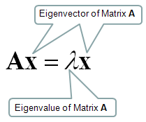
The eigenvector is also known as the characteristic vector. It is a non-zero vector that only changes with the scalar factor when a linear transformation is applied to it.
Eigenvectors are rotational axes of the linear transformation. These axes are fixed in direction, and eigenvalue is the scale factor by which the matrix is scaled up or down. Eigenvalues are also known as characteristic values or characteristic roots. In other words, you can say eigenvalues are fixed line or plane which limits the behavior of the linear transformation and eigenvalues of a linear transformation are the factor of distortion.
Determinant tells you the area of shapes that scaled up and down in linear transformation. That's why the multiplication of eigenvalues is equal to the determinant.
# Import numpy module
import numpy as np

# Create 2*2 matrix
arr=np.array([[1,2],[3,4]])

# Find eigenvalues and eigenvectors
eigenvalues, eigenvectors = np.linalg.eig(arr)

# print the eigenvalues and eigenvectors
print("Eigen Values: \n",eigenvalues)
print("Eigen Vectors:\n", eigenvectors)
Eigen Values:
 [-0.37228132  5.37228132]
Eigen Vectors:
 [[-0.82456484 -0.41597356]
 [ 0.56576746 -0.90937671]]
NORM Function
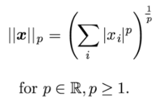
Sometimes you want to measure the size of a vector. Norm function helps you measure the size of a vector. It assigns a strict positive length to a vector in a vector space except for zero vector. It includes the L^p norm. It maps vectors to non-negative values. It is equivalent to Euclidean distance for a vector and a matrix. It is equal to the largest singular value.
# import numpy module
import numpy as np

# Create 3*3 Matrix
a = np.array([[1,2,3],[4,5,6],[7,8,9]])

# Compute norm
a_norm = np.linalg.norm(a)

# print the norm of function
print(a_norm)
16.881943016134134
Matrix Factorization
Matrix factorization, also known as matrix decomposition. It is used to split a matrix into its constituent parts. Matrix factorization is equivalent to the factoring of numbers, such as the factoring of 10 into 2 x 5. It is used to solve linear equations.
The following matrix factorization techniques are available:
- LU Decomposition is for square matrices and decomposes a matrix into L and U components.
- QR Decomposition is for m x n matrices (not limited to square matrices) and decomposes a matrix into Q and R components. It is not limited to square matrices like LU decomposition.
- Cholesky Decomposition is used for solving linear least squares for linear regression, as well as simulation and optimization methods.
- Singular Value Decomposition explained in the next section.
Singular Value Decomposition
In the previous section, we have seen eigen-decomposition of a matrix that decomposes into eigenvectors and eigenvalues. Singular value decomposition is a type of matrix factorization method that decomposes into singular vectors and singular values. It offers various useful applications in signal processing, psychology, sociology, climate, atmospheric science, statistics, and astronomy.

- M is an m×m matrix
- U is a m×n left singular matrix
- Σ is a n×n diagonal matrix with non-negative real numbers.
- V is a m×n right singular matrix
- V* is n×m matrix, which is the transpose of the V.
# Import numpy module
import numpy as np

# Create 3*3 matrix
a = np.array([[1, 3, 4], [5, 6, 9], [1, 2, 3], [7, 6, 8]])

# Decomposition of matrix using SVD
U, s, Vh = np.linalg.svd(a, full_matrices=False)

U,s,Vh
(array([[-0.27067357, -0.61678044,  0.69789573],
        [-0.65939972, -0.2937857 , -0.62152182],
        [-0.20244298, -0.3480035 , -0.06765408],
        [-0.67152413,  0.64200111,  0.34939247]]),
 array([18.0376394 ,  2.34360292,  0.38870323]),
 array([[-0.46961711, -0.51018039, -0.72053851],
        [ 0.87911451, -0.19502274, -0.43488368],
        [-0.08134773,  0.83766467, -0.54009299]]))
# Generate the initial matrix
new_a = np.dot(U, np.dot(np.diag(s), Vh))

# Print original matrix
print(new_a)
[[1. 3. 4.]
 [5. 6. 9.]
 [1. 2. 3.]
 [7. 6. 8.]]
Moore-Penrose Pseudoinverse
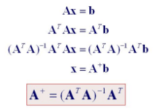
Pseudoinverse of a matrix is generalized of the inverse matrix. It is utilized in computing the least square solutions. Moore-Penrose inverse is the most popular form of matrix pseudoinverse.
# Import numpy module
import numpy as np

# Create 3*3 matrix
a = np.array([[1, 3, 4], [5, 6, 9], [1, 2, 3], [7, 6, 8]])

# Compute the (Moore-Penrose) pseudo-inverse of a matrix.
inv=np.linalg.pinv(a)

# Print pseudo-inverse of a matrix.
print(inv)
[[-0.37037037  0.03703704 -0.11111111  0.18518519]
 [ 1.56296296 -1.2962963  -0.11111111  0.71851852]
 [-0.84444444  0.94444444  0.16666667 -0.57777778]]
Hadamard Product
Hadamard product or Schur product is an element-wise product of two same dimensional original matrices. It is also known as the element-wise product. It is simpler than the matrix product. Hadamard product is utilized in JPEG lossy compression algorithms. Hadamard product is commutative, associative, and distributive. It easily obtains the inverse and simplifies the computation of power matrices.

Hadamard product is utilized in various fields such as code correction in satellite transmissions, information theory, cryptography, pattern recognition, neural network, maximum likelihood estimation, JPEG lossy compression, multivariate statistical analysis, and linear modeling.
# Import numpy module
import numpy as np

# Create 2*2 matrix a1 and a2
a1=np.array([[1, 2], [3, 4]])
a2=np.array([[1, 2], [3, 4]])

# Element wise multiplication
hadamard_product = np.multiply(a1,a2)

# Print hadamard distance
print("Hadamard Product: \n", hadamard_product)
Hadamard Product:
 [[ 1  4]
 [ 9 16]]
Entropy
"The entropy of a random variable is a function which attempts to characterize the unpredictability of a random variable." (Entropy and Mutual Information)" It is used for the construction of an automatic decision tree at each step of tree building; feature selection is done such using entropy criteria. Model selection is based on the principle of the maximum entropy, which states from the conflicting models, the one with the highest entropy is the best.
"If a random variable X takes on values in a set χ={x1, x2,..., xn}, and is defined by a probability distribution P(X), then we will write the entropy of the random variable as," (Entropy and Mutual Information)

"If the log in the above equation is taken to be to the base 2, then the entropy is expressed in bits. If the log is taken to be the natural log, then the entropy is expressed in nats. More commonly, entropy is expressed in bits." (Entropy and Mutual Information)
# Import scipy and numpy module
import scipy.stats
import numpy as np

# Create an array
a=np.array([1,1,2,3,1,3,4,2,5,6,3,2,4,3])


# Compute probability distribution
a_pdf=scipy.stats.norm.pdf(a)

# Calculate the entropy of a distribution for given probability values.
entropy = scipy.stats.entropy(a_pdf) # get entropy from probability values
print("Entropy: ",entropy)
Entropy: 1.6688066853941022
Kullback-Leibler Divergence
Kullback–Leibler divergence is the relative entropy of two probability distributions. It measures the distance(similarity or dissimilarity) of one distribution from another reference probability distribution. 0 Value of Kullback–Leibler divergence indicates that both distributions are identical. It can be expressed as,

It does sound like a distance measure, but it is not. This is because it is asymmetric in nature, which means the metric isn’t commutative. In general, you can say that D(p, q) ≠D(q, p). KL divergence is frequently used in the un-supervised machine learning technique “Variational Autoencoders”.
# Import scipy.stats and numpy module
import scipy.stats
import numpy as np

# Create numpy arrays
a=np.array([1,1,2,3,1,3,4,2,5,6,3,2,4,3])
b=np.array([1,1,3,4,2,4,5,2,5,6,3,2,4,3])

# Compute probability distribution
a_pdf=scipy.stats.norm.pdf(a)
b_pdf=scipy.stats.norm.pdf(b)

# compute relative entropy or KL Divergence
kl_div=scipy.stats.entropy(a_pdf,b_pdf)

print("KL Divergence: ",kl_div)
KL Divergence: 0.26732496641464365
Gradient Descent
Gradient descent is one of the most well-known algorithms used to optimize coefficients and bias for linear regression, logistic regression, and neural networks. It is an iterative process that finds the minimum of any given function.
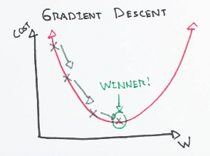

Three types of the gradient descent algorithm: full batch, stochastic, and mini-batch gradient descent. Full batch gradient descent uses the whole dataset for computing gradient while stochastic gradient descent uses a sample of the dataset for computing gradient. Mini-batch gradient descent is a combination of both stochastic and batch gradient descent. The training set is split into various small groups called batches. These small batches compute the loss one by one and average the final loss result.
Conclusion
Congratulations, you have made it to the end of this tutorial!
You learned basic mathematical concepts for deep learning such as scalar, vector, matrix, tensor, determinant eigenvalues, eigenvectors, NORM function, singular value decomposition(SVD), Moore-Penrose Pseudoinverse, Hadamard product, Entropy Kullback-Leibler Divergence, and Gradient Descent.
Along the road, you have also practiced these concepts in python using NumPy and SciPy.
If you would like to learn more about Python, take the following DataCamp courses:


