Data visualization is an essential skill for data scientists. It combines statistics and design in meaningful and appropriate ways. On the one hand, data visualization is a form of graphical data analysis, emphasizing accurate representation, and data interpretation. On the other hand, data visualization relies on good design choices to make our plots attractive and aid both the understanding and communication of results. On top of that, there is an element of creativity, since data visualization is a form of visual communication at its heart.
It's important to understand the distinction between exploratory and explanatory visualizations. Exploratory visualizations are easily-generated, data-heavy, and intended for a small specialist audience, such as yourself and your colleagues - their primary purpose is graphical data analysis. Explanatory visualizations are labor-intensive, data-specific, and intended for a broader audience, e.g., in publications or presentations - they are part of the communications process. As a data scientist, it's essential that you can quickly explore data, but you'll also be tasked with explaining your results to stake-holders. Good design begins with thinking about the audience - and sometimes that just means ourselves.
Scatter Plot
Below, we have a dataset that contains the average brain and body weights of 62 mammals.
Applying a log transformation of both variables allows for a better fit.
ggplot(mammals,aes(x = body, y = brain))+geom_point(alpha =0.6)+coord_fixed()+scale_x_log10()+scale_y_log10()+stat_smooth(
method ="lm",
color ="#C42126",
se =FALSE,
size =1)
So, although we began with a rough exploratory plot, it informed us about our data and led us to a meaningful result.
Anscombe's Plots
When we imagine a linear model, as presented on this anonymous plot, we imagine that we are describing data that looks something like this.
But this same model could be describing a very different set of data, such as a parabolic relationship, which calls for a different model.
Or data in which an extreme value has a large effect. which becomes clear when the outlier is removed.
And sometimes, the model may be describing a relationship where, in fact, there is none at all because some extreme values may be incorrect.
If we relied solely on the numerical output without plotting our data, we'd have missed distinct and interesting underlying trends.
We can see that data visualization is rooted in statistics and graphical data analysis, but it's also a creative process that involves some amount of trial and error.
Interactive Example
In the following example, you will first Load the ggplot2 package using library(). Then, you will use str() to explore the structure of the mtcars dataset.
Finally, you will visualize the ggplot and try to understand what ggplot does with the data.
You will use the mtcars dataset contains information on 32 cars from a 1973 issue of Motor Trend magazine. This dataset is small, intuitive, and contains a variety of continuous and categorical variables.
# Load the ggplot2 package
library(ggplot2)# Explore the mtcars data frame with str()str(mtcars)# Execute the following command
p <- ggplot(mtcars, aes(cyl, mpg))+
geom_point()
When we run the above code, it produces the following result:
data.frame':32 obs.of11variables:
$ mpg : num 212122.821.418.718.114.324.422.819.2...
$ cyl : num 6646868446...
$ disp: num 160160108258360...
$ hp : num 110110931101751052456295123...
$ drat: num 3.93.93.853.083.152.763.213.693.923.92...
$ wt : num 2.622.882.323.213.44...
$ qsec: num 16.51718.619.417...
$ vs : num 0011010111...
$ am : num 1110000000...
$ gear: num 4443333444...
$ carb: num 4411214224...
Learn what data visualization is and why it is an essential skill for data scientists. Discover the numerous ways you can visualize your data and boost your storytelling skills.
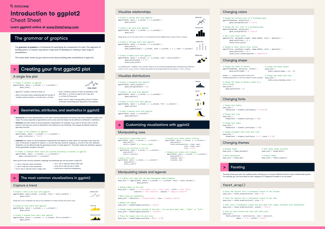
ggplot2 is considered to be one of the most robust data visualization packages in any programming language. Use this cheat sheet to guide your ggplot2 learning journey.
Learn how to use ggplot2 in R to create compelling visualizations of climate change data. This step-by-step tutorial teaches you to find, analyze, and visualize historical weather data.



 Kurtis Pykes · 15 min
 Richie Cotton

 Bruno Ponne · 11 min



Data visualization is an essential skill for data scientists. It combines statistics and design in meaningful and appropriate ways. On the one hand, data visualization is a form of graphical data analysis, emphasizing accurate representation, and data interpretation. On the other hand, data visualization relies on good design choices to make our plots attractive and aid both the understanding and communication of results. On top of that, there is an element of creativity, since data visualization is a form of visual communication at its heart.
It's important to understand the distinction between exploratory and explanatory visualizations. Exploratory visualizations are easily-generated, data-heavy, and intended for a small specialist audience, such as yourself and your colleagues - their primary purpose is graphical data analysis. Explanatory visualizations are labor-intensive, data-specific, and intended for a broader audience, e.g., in publications or presentations - they are part of the communications process. As a data scientist, it's essential that you can quickly explore data, but you'll also be tasked with explaining your results to stake-holders. Good design begins with thinking about the audience - and sometimes that just means ourselves.
Scatter Plot
Below, we have a dataset that contains the average brain and body weights of 62 mammals.
To understand the relationship here, the most obvious first step is to make a scatter plot, like the one shown below:
Two mammals, the African and the Asian Elephants have both very large brain and body weights, leading to a positive skew on both axes.
Linear Model
Now, if we were to apply a linear model, it would be a poor choice since a few extreme values have a large influence.
Applying a log transformation of both variables allows for a better fit.
So, although we began with a rough exploratory plot, it informed us about our data and led us to a meaningful result.
Anscombe's Plots
When we imagine a linear model, as presented on this anonymous plot, we imagine that we are describing data that looks something like this.
But this same model could be describing a very different set of data, such as a parabolic relationship, which calls for a different model.
Or data in which an extreme value has a large effect. which becomes clear when the outlier is removed.
And sometimes, the model may be describing a relationship where, in fact, there is none at all because some extreme values may be incorrect.
If we relied solely on the numerical output without plotting our data, we'd have missed distinct and interesting underlying trends.
We can see that data visualization is rooted in statistics and graphical data analysis, but it's also a creative process that involves some amount of trial and error.
Interactive Example
In the following example, you will first Load the
ggplot2package using library(). Then, you will use str() to explore the structure of themtcarsdataset.Finally, you will visualize the ggplot and try to understand what ggplot does with the data.
You will use the
mtcarsdataset contains information on 32 cars from a 1973 issue of Motor Trend magazine. This dataset is small, intuitive, and contains a variety of continuous and categorical variables.When we run the above code, it produces the following result:
To learn more about data visualization with ggplot, please see this video from our course Introduction to Data Visualization with ggplot2. Also, keep our ggplot2 Cheat Sheet close by as a handy reference.
This content is taken from DataCamp’s Introduction to Data Visualization with ggplot2 course by Rick Scavetta.