Facets for ggplot2 in R

Introduction

With facetting, you can make multi-panel plots and control how the scales of one panel relate to the scales of another.

Simple Facet Usage

If you're at all familiar with ggplot2, you'll know the basic structure of a call to the ggplot() function. For an introduction to ggplot2, you can check out our  ggplot2 course. When you call ggplot, you provide a data source, usually a data frame, then ask ggplot to map different variables in our data source to different aesthetics, like the position of the x or y-axes or the color of our points or bars. With facets, you gain an additional way to map the variables. To demonstrate this, you'll make use of the following dataset, which includes a number of economic indicators for a selection of countries. Most of these are variants on GDP, the Gross Domestic Product of each country.

 print(econdata)

##   Country  GDP_nom  GDP_PPP GDP_nom_per_capita GDP_PPP_per_capita
## 1     USA 19390600 19390600              59501              59495
## 2  Canada  1652412  1769270              45077              48141
## 3   China 12014610 23159107               8643              16807
## 4   Japan  4872135  5428813              38440              42659
## 5  France  2583560  2835746              39869              43550
## 6 Germany  3684816  4170790              44550              50206
## 7  Sweden  3684816   520937              53218              51264
## 8 Ireland   333994   343682              70638              72632
##   GNI_per_capita        Region
## 1          58270 North America
## 2          42870 North America
## 3           8690          Asia
## 4          38550          Asia
## 5          37970        Europe
## 6          43490        Europe
## 7          52590        Europe
## 8          55290        Europe

The following variables are present:

Country: Self-explanatory!

GDP_nom: Gross Domestic Product as a nominal value in USD

GDP_PPP: Gross Domestic Product controlled for differing purchasing power

GDP_nom_per_capita: Gross Domestic Product as a nominal value in USD on a per capita basis

GDP_PPP_per_capita: Gross Domestic Product controlled for differing purchasing power on a per capita basis

GNI_per_capita: Gross National Income for each country on a per capita basis.

Region: region of the world where the country is located.

To start with, let's make a simple barplot of the nominal GDP of each country.

ggplot(econdata, aes(x=Country, y=GDP_nom))+
  geom_bar(stat='identity', fill="forest green")+
  ylab("GDP (nominal)")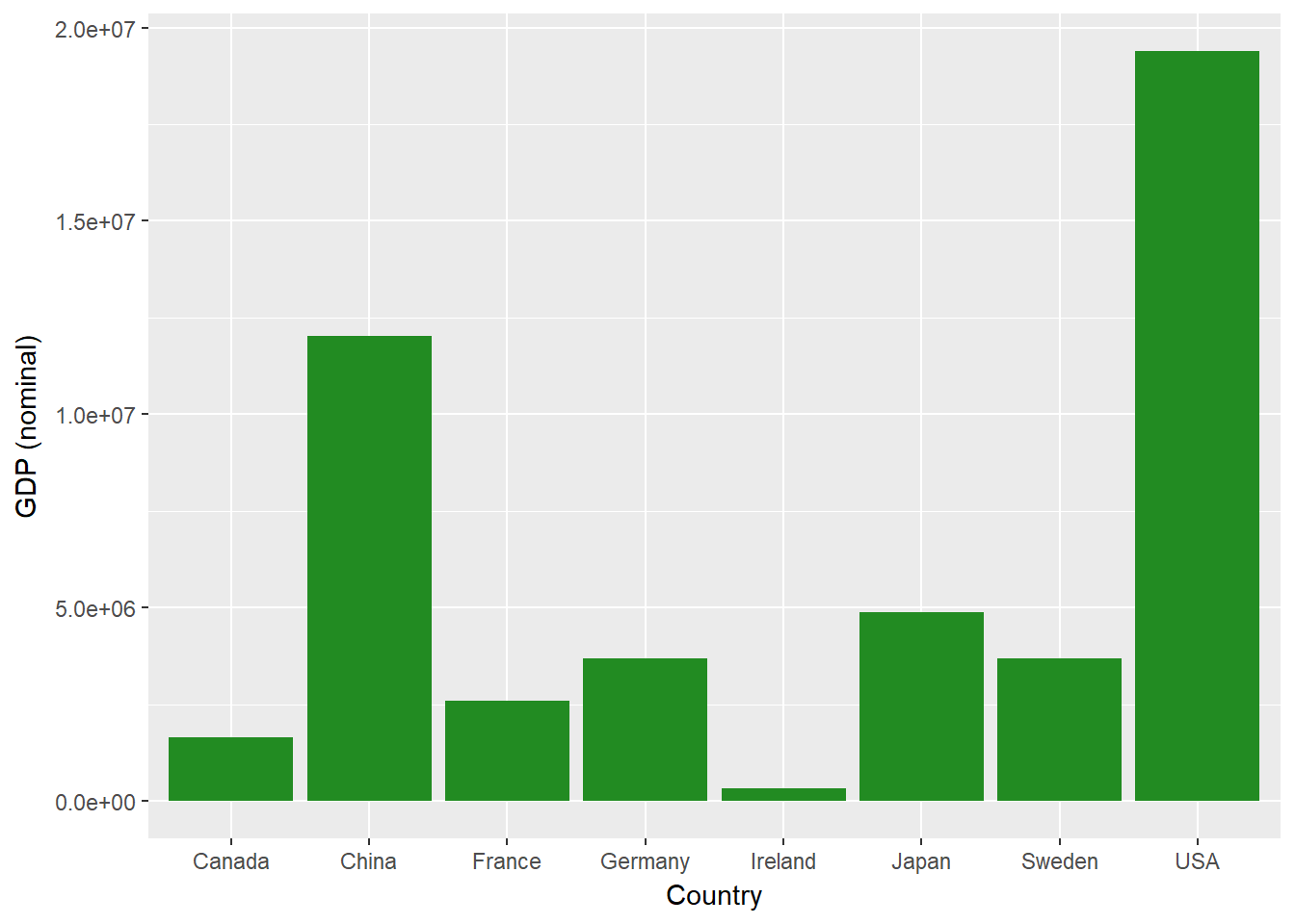

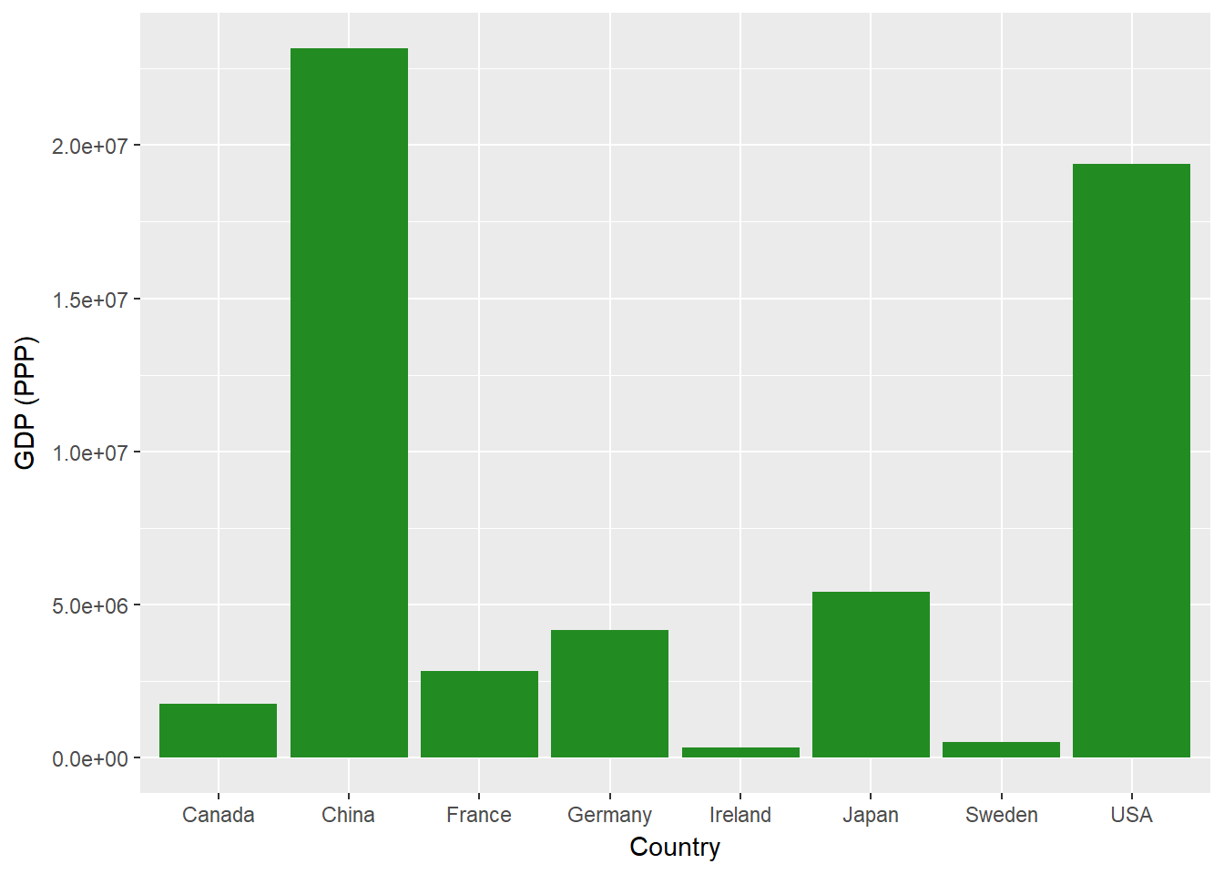
You can also plot another variable, the PPP-adjusted GDP.

ggplot(econdata, aes(x=Country, y=GDP_PPP))+
  geom_bar(stat='identity', fill="forest green")+
  ylab("GDP (PPP)")

This gives you a second separate graph, similar to the last but making use of a different variable. Let's say you want to plot both GDP (nominal) and GDP (PPP) together. You'll use facetting to do so. First, you'll need to reformat your data, changing it from a "wide" format with each variable in its own column to a "long" format, where you use one column for your measures and another for a key variable telling us which measure we use in each row.

econdatalong <- gather(econdata, key="measure", value="value", c("GDP_nom", "GDP_PPP"))

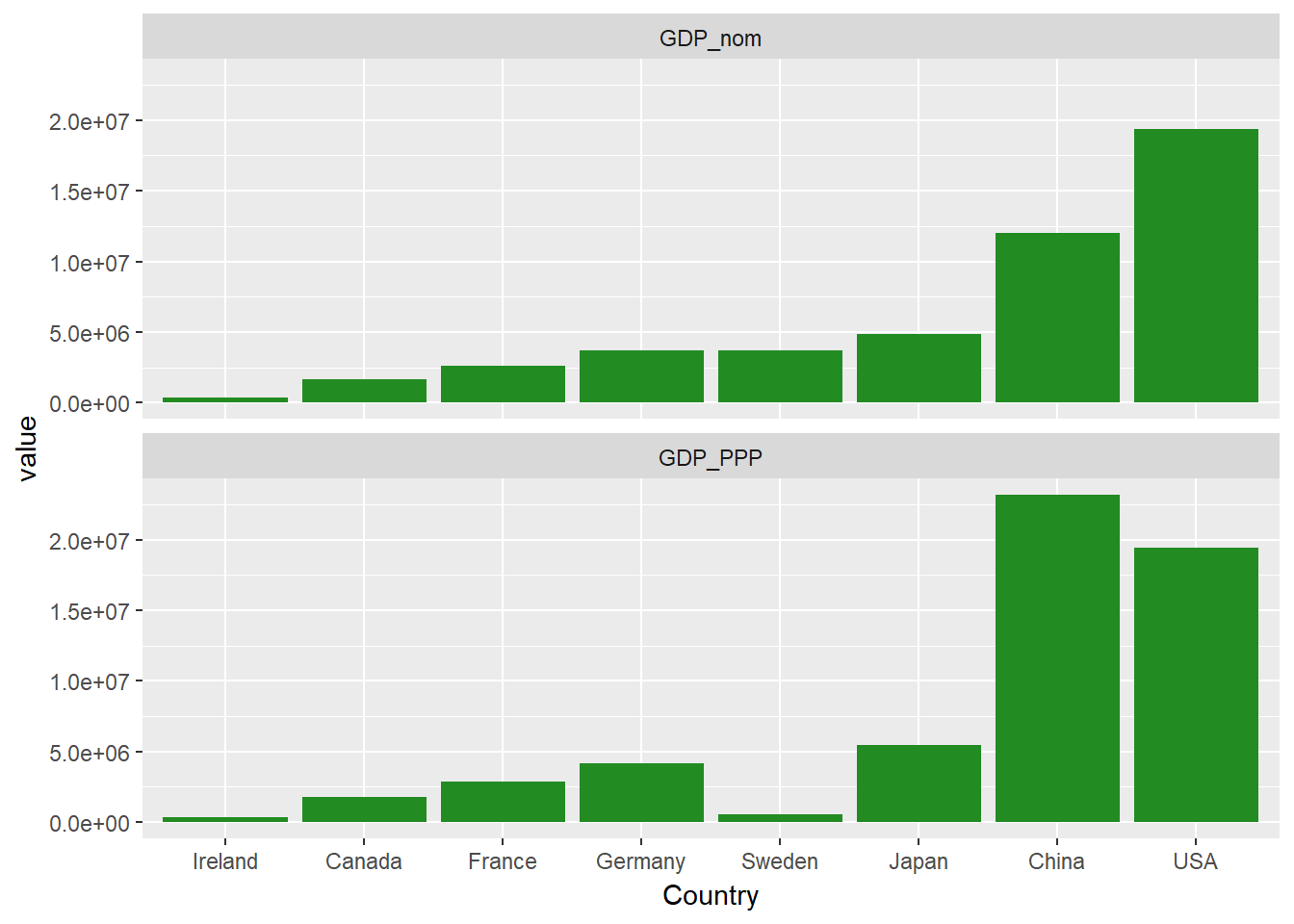
Once you have the data in such a format, you can then make use of our key variable in order to plot with facets. Let's build a simple plot, showing both nominal GDP (from our first plot) and GDP (PPP) (from our second plot). In order to do so, you simply modify your code to add +facet_wrap() and specify that ~measure, our key variable, should be used for facetting.

ggplot(econdatalong, aes(x=Country, y=value))+
  geom_bar(stat='identity', fill="forest green")+
  facet_wrap(~measure)

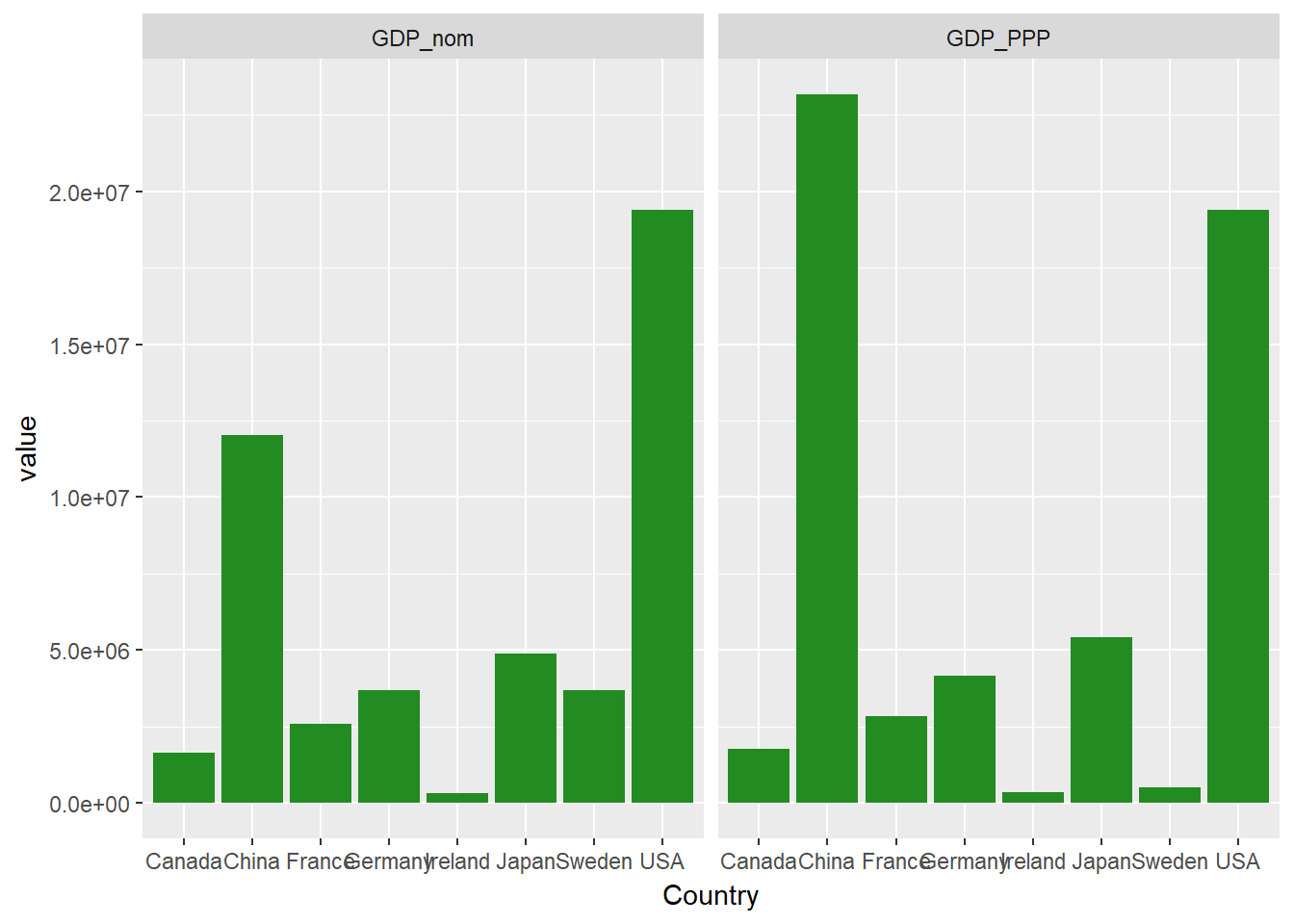
This works, but you'll notice how squashed the country names are. Let's rearrange our panels.

Customizing Layout and re-ordering

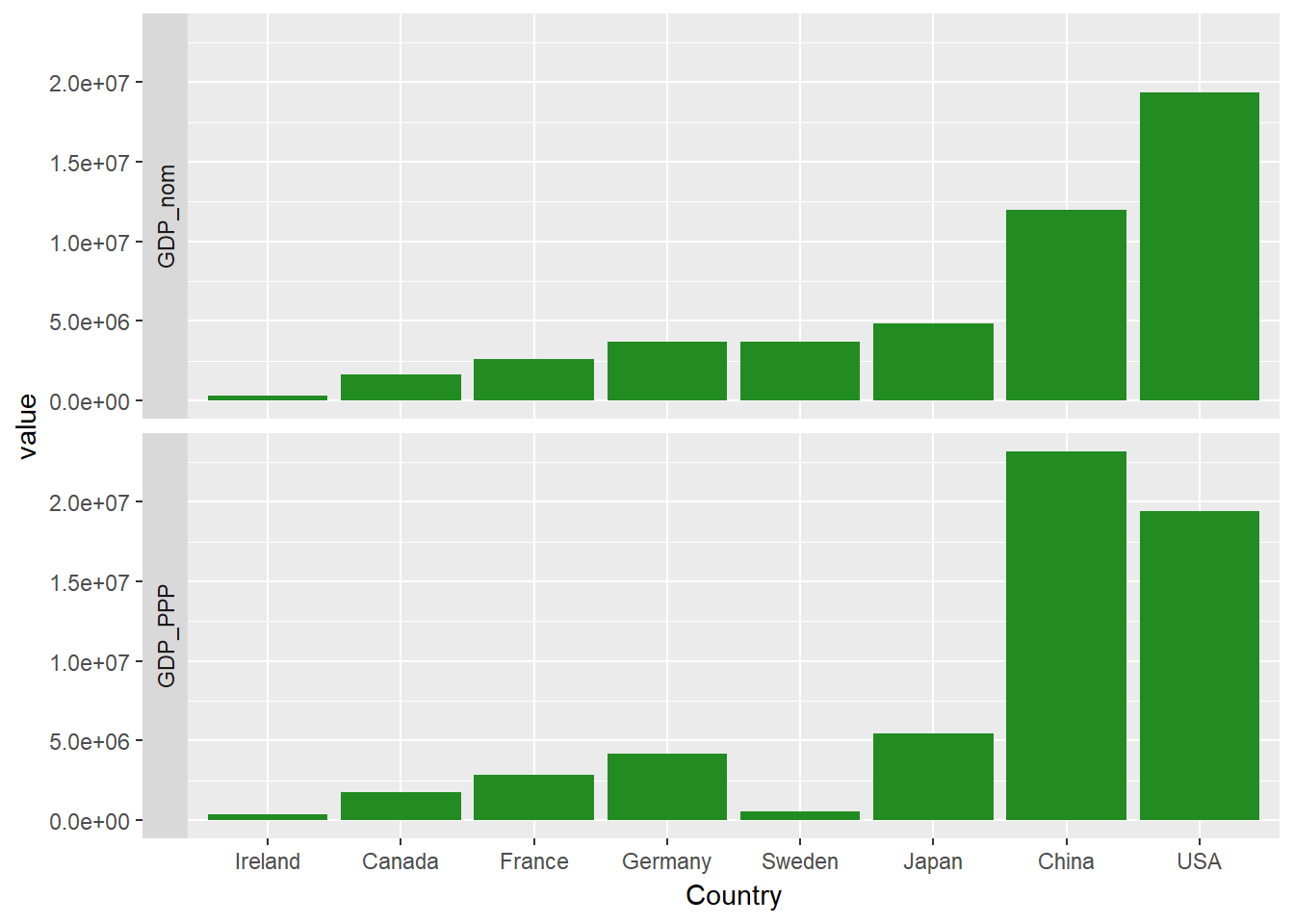
The facet_wrap() command will automatically choose how many columns to use. You can specify this directly using ncol=, like so:

ggplot(econdatalong, aes(x=Country, y=value))+
  geom_bar(stat='identity', fill="forest green")+
  facet_wrap(~measure,  ncol=1)

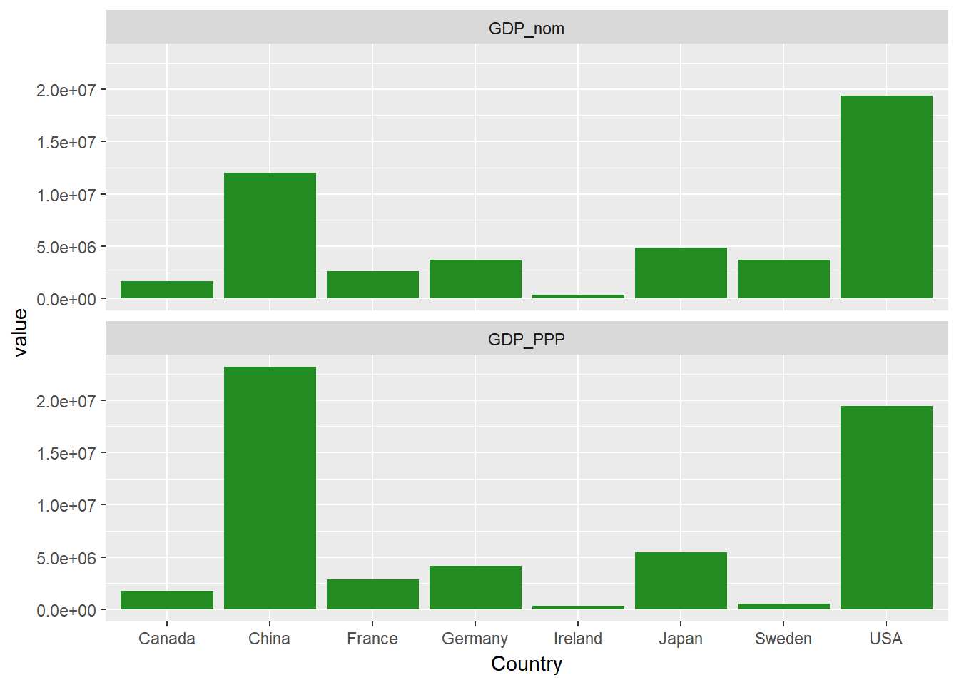
You probably notice that the countries, on the x-axis above, are arranged in alphabetical order. If you want to change this, the easiest way to do so is to set the levels of the Country factor. Let's perform this re-ordering, arranging the countries in order of total nominal GDP.

econdata$Country <- factor(econdata$Country, levels= econdata$Country[order(econdata$GDP_nom)])


econdatalong <- gather(econdata, key="measure", value="value", c("GDP_nom", "GDP_PPP"))


ggplot(econdatalong, aes(x=Country, y=value))+
  geom_bar(stat='identity', fill="forest green")+
  facet_wrap(~measure,  ncol=1)

You can also do some extra customization, like moving the facet labels to the left-hand side with the strip.position argument.

ggplot(econdatalong, aes(x=Country, y=value))+
  geom_bar(stat='identity', fill="forest green")+
  facet_wrap(~measure,  ncol=1, strip.position = "left")

Labelling Facets

You may have noticed that the facets have simple short headings, taken from the levels of the factor measure. Let's tidy this up and give our facets some nicer labels. To do this, you'll make a simple labeller function, variable_labeller, which will return the appropriate name when asked for one of the values of variable_names. Then, you pass this function to the labeller argument of facet_wrap.

variable_names <- list(
  "GDP_nom" = "GDP (nominal)" ,
  "GDP_PPP" = "GDP (purchasing power parity)"
)


variable_labeller <- function(variable,value){
  return(variable_names[value])
}


ggplot(econdatalong, aes(x=Country, y=value))+
  geom_bar(stat='identity', fill="forest green")+
  facet_wrap(~measure,  ncol=1, labeller=variable_labeller)

Playing with Scales and Space

Let's build a larger faceted plot, using each of the economic measures.

econdatalong <- gather(econdata, key="measure", value="value", c( "GDP_nom" , "GDP_PPP" ,"GDP_nom_per_capita", "GDP_PPP_per_capita" ,"GNI_per_capita"))

variable_names <- list(
  "GDP_nom" = "GDP (nominal)" ,
  "GDP_PPP" = "GDP (purchasing power parity)",
  "GDP_nom_per_capita" = "GDP (nominal) per capita",
  "GDP_PPP_per_capita" = "GDP (purchasing power parity) per capita",
  "GNI_per_capita"  = "GNI per capita"
)


variable_labeller <- function(variable,value){
  return(variable_names[value])
}



ggplot(econdatalong, aes(x=Country, y=value))+
  geom_bar(stat='identity', fill="forest green")+
  facet_wrap(~measure,  ncol=1, labeller= variable_labeller)+
scale_y_continuous(breaks = pretty(econdatalong$value, n = 10))

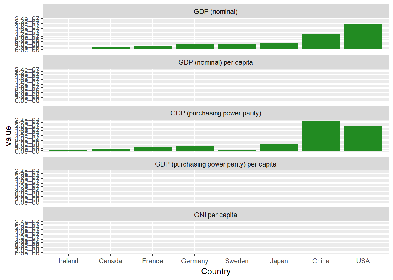
That's no good at all! You can't see the values for three of the panels. Why is that? Let's have a look at the primary data to see why.

summary(econdata)

##     Country     GDP_nom            GDP_PPP         GDP_nom_per_capita
##  Ireland:1   Min.   :  333994   Min.   :  343682   Min.   : 8643     
##  Canada :1   1st Qu.: 2350773   1st Qu.: 1457187   1st Qu.:39512     
##  France :1   Median : 3684816   Median : 3503268   Median :44814     
##  Germany:1   Mean   : 6027118   Mean   : 7202368   Mean   :44992     
##  Sweden :1   3rd Qu.: 6657754   3rd Qu.: 8919260   3rd Qu.:54789     
##  Japan  :1   Max.   :19390600   Max.   :23159107   Max.   :70638     
##  (Other):2                                                           
##  GDP_PPP_per_capita GNI_per_capita            Region
##  Min.   :16807      Min.   : 8690   Asia         :2  
##  1st Qu.:43327      1st Qu.:38405   Europe       :4  
##  Median :49174      Median :43180   North America:2  
##  Mean   :48094      Mean   :42215                    
##  3rd Qu.:53322      3rd Qu.:53265                    
##  Max.   :72632      Max.   :58270                    
##

If you have a look at each column, you see that the values in each column range over a few orders of magnitude. By default, facetting will use the same limits and ranges for both the X and Y-axes. To change this, you can add this snippet to your facetting code: scales="free_y" so that each facet will use its own independent scale.

ggplot(econdatalong, aes(x=Country, y=value))+
  geom_bar(stat='identity', fill="forest green")+
  facet_wrap(~measure, scales="free_y", ncol=1,  labeller= variable_labeller)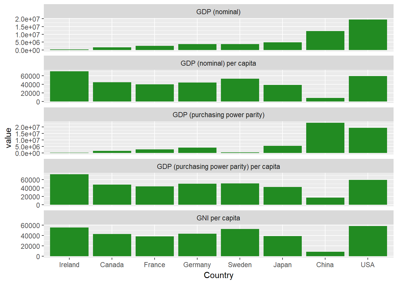

This is much better. Each facet now has its own independent y-axis.

Using Facets to Create Subdivisions

You may have noticed that our dataset also includes the variable Region, which denotes what region the country in question is located. You can use this variable to color our bars according to region, as follows:

ggplot(econdatalong, aes(x=Country, y=value, fill=Region))+
  geom_bar(stat='identity')+
  facet_wrap(~measure, scales="free_y", ncol=1, labeller= variable_labeller)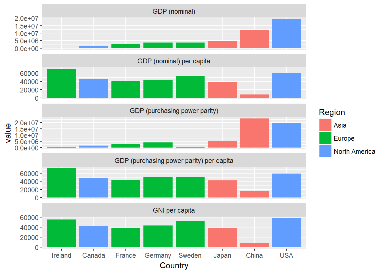

However, this is a little messy, wouldn't it be nice if you could put each of the different regions in their own sub-panel? Well, with facetting, you can! Here you're going to use facet_grid instead of facet_wrap, as that will make it easy to map our facets to two variables, Region and measure, where all these two variables are spread across the rows and columns of a grid of plots. Note that you are also setting scales="free" and space="free", allowing our different panels to take up different amounts of space. You'll also need to create a new labeller function, which will produce names for both rows and labels.

variable_names <- list(
  "GDP_nom" = "GDP \n(nominal)" ,
  "GDP_PPP" = "GDP \n(PPP)",
  "GDP_nom_per_capita" = "GDP (nominal)\n per capita",
  "GDP_PPP_per_capita" = "GDP (PPP)\n per capita",
  "GNI_per_capita"  = "GNI \nper capita"
)



region_names <- levels(econdata$Region)


variable_labeller2 <- function(variable,value){
  if (variable=='measure') {
  return(variable_names[value])
  } else {
    return(region_names)
  }
}

ggplot(econdatalong, aes(x=Country, y=value, fill=Region))+
  geom_bar(stat='identity')+
  facet_grid(measure~Region, scales="free", space="free_x",  labeller= variable_labeller2)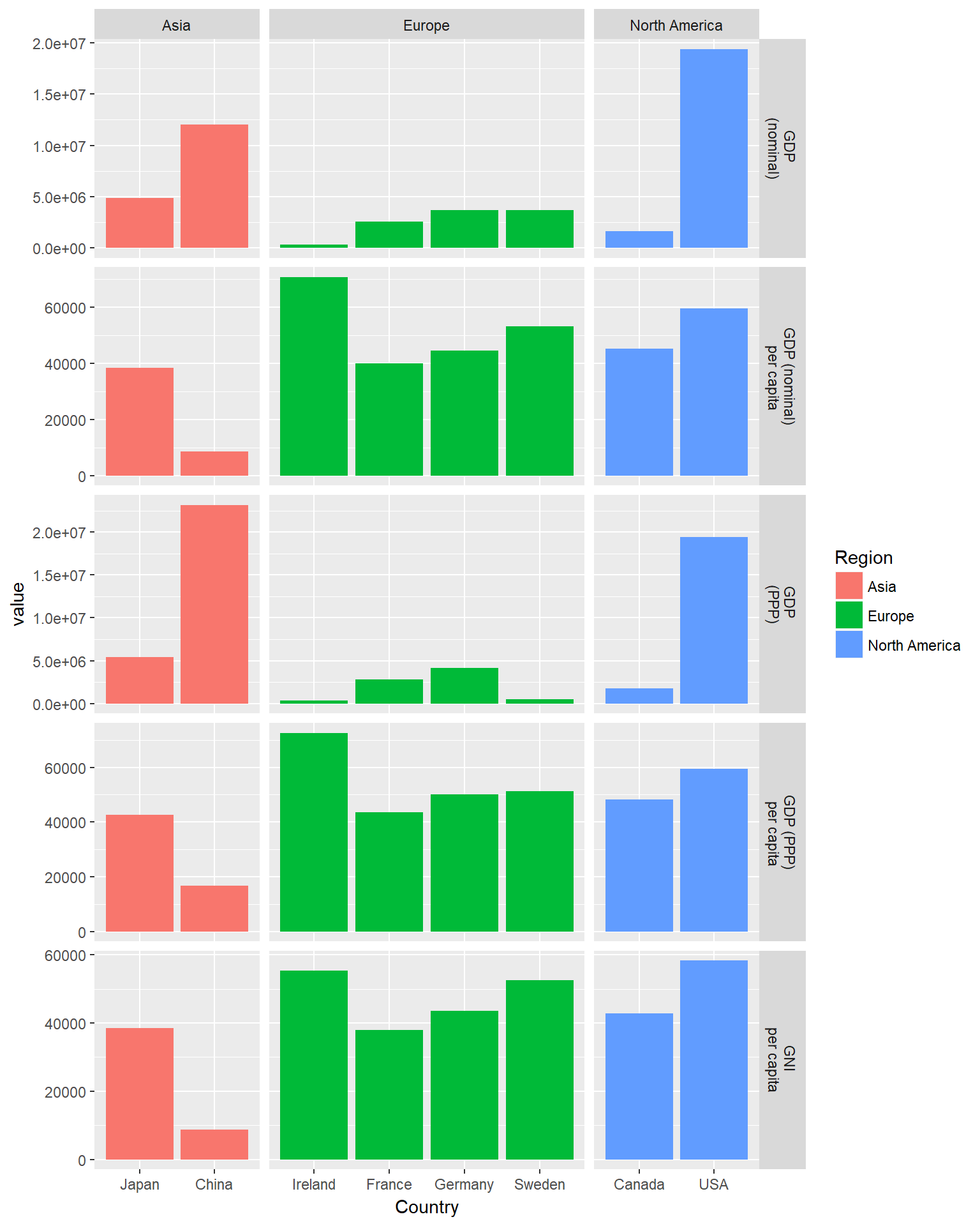

Now it's much clearer! Each region has its own column of panels, and each metric has its own row of bars.

That about wraps it up for this tutorial. I hope you enjoyed learning about facets.

If you would like to learn more about facets, take DataCamp's Visualizing Big Data with Trelliscope course.

Check out our Getting Started with the Tidyverse: Tutorial.