R Highcharter 用于 Highcharts 数据可视化

我认为数据可视化是展示一组数据的描述性与分析性报告的最佳方式。我个人非常热爱数据可视化。您可以在单个屏幕中讲完整个故事——当然这也取决于数据的复杂度。如果您在阅读本教程，我想您应该了解过 R 中的 Ggplot2 包，它能生成非常出色的分析图表，但在动态特性方面略显不足。

回到 Highcharter，它是 HighCharts JavaScript 库及其模块的 R 封装。

该包的主要特性包括：

以统一风格创建多种图表，如散点图、气泡图、时间序列、热力图、矩形树图、条形图等。
支持多种 R 对象。
支持 Highstocks 图表与分级着色地图（Choropleths）。
采用 R 用户与程序员都喜爱的管道（piping）风格。
提供大量外观出色的主题。

接下来让我们开工，结合上述特性，用 Highcharter 创建一些可视化：

使用 hchart 函数创建一些基础图表

hchart 是一个泛型函数，它接收一个对象并返回一个 highcharter 对象。有些函数的行为与 ggplot2 包中的函数类似：

hchart 类似于 ggplot2 的 qplot。
hc_add_series 类似于 ggplot2 的 geom_S。
hcaes 类似于 ggplot2 的 aes。

我们选择一个数据集。我将使用 Highcharter 包中提供的 Pokemon 数据集。先快速浏览一下数据集。

glimpse(pokemon)技术支持

## Observations: 718
## Variables: 20
## $ id              <dbl> 1, 2, 3, 4, 5, 6, 7, 8, 9, 10, 11, 12, 13, 14,...
## $ pokemon         <chr> "bulbasaur", "ivysaur", "venusaur", "charmande...
## $ species_id      <int> 1, 2, 3, 4, 5, 6, 7, 8, 9, 10, 11, 12, 13, 14,...
## $ height          <int> 7, 10, 20, 6, 11, 17, 5, 10, 16, 3, 7, 11, 3, ...
## $ weight          <int> 69, 130, 1000, 85, 190, 905, 90, 225, 855, 29,...
## $ base_experience <int> 64, 142, 236, 62, 142, 240, 63, 142, 239, 39, ...
## $ type_1          <chr> "grass", "grass", "grass", "fire", "fire", "fi...
## $ type_2          <chr> "poison", "poison", "poison", NA, NA, "flying"...
## $ attack          <int> 49, 62, 82, 52, 64, 84, 48, 63, 83, 30, 20, 45...
## $ defense         <int> 49, 63, 83, 43, 58, 78, 65, 80, 100, 35, 55, 5...
## $ hp              <int> 45, 60, 80, 39, 58, 78, 44, 59, 79, 45, 50, 60...
## $ special_attack  <int> 65, 80, 100, 60, 80, 109, 50, 65, 85, 20, 25, ...
## $ special_defense <int> 65, 80, 100, 50, 65, 85, 64, 80, 105, 20, 25, ...
## $ speed           <int> 45, 60, 80, 65, 80, 100, 43, 58, 78, 45, 30, 7...
## $ color_1         <chr> "#78C850", "#78C850", "#78C850", "#F08030", "#...
## $ color_2         <chr> "#A040A0", "#A040A0", "#A040A0", NA, NA, "#A89...
## $ color_f         <chr> "#81A763", "#81A763", "#81A763", "#F08030", "#...
## $ egg_group_1     <chr> "monster", "monster", "monster", "monster", "m...
## $ egg_group_2     <chr> "plant", "plant", "plant", "dragon", "dragon",...
## $ url_image       <chr> "1.png", "2.png", "3.png", "4.png", "5.png", "...技术支持

我们来绘制一个条形图。

pokemon%>%
  count(type_1)%>%
  arrange(n)%>%
  hchart(type = "bar", hcaes(x = type_1, y = n))技术支持

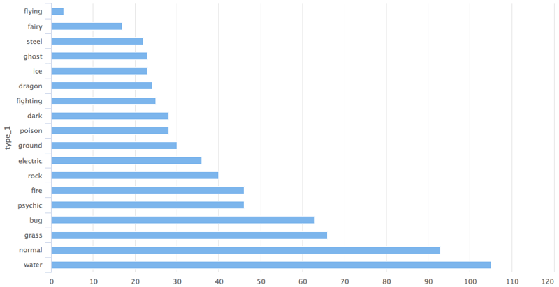
这样您就得到了一个关于宝可梦 type 1 分类的条形图。

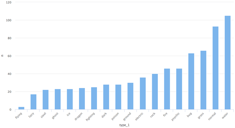
如果您想要改为柱状图，只需将类型改为 column 即可。

pokemon%>%
  count(type_1)%>%
  arrange(n)%>%
  hchart(type = "column", hcaes(x = type_1, y = n))技术支持

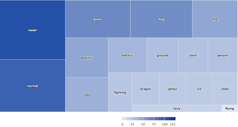
矩形树图

pokemon%>%
  count(type_1)%>%
  arrange(n)%>%
  hchart(type = "treemap", hcaes(x = type_1, value = n, color = n))技术支持

我们也可以用 hc_add_series 来绘图。它用于在 highchart 对象中添加或移除系列。

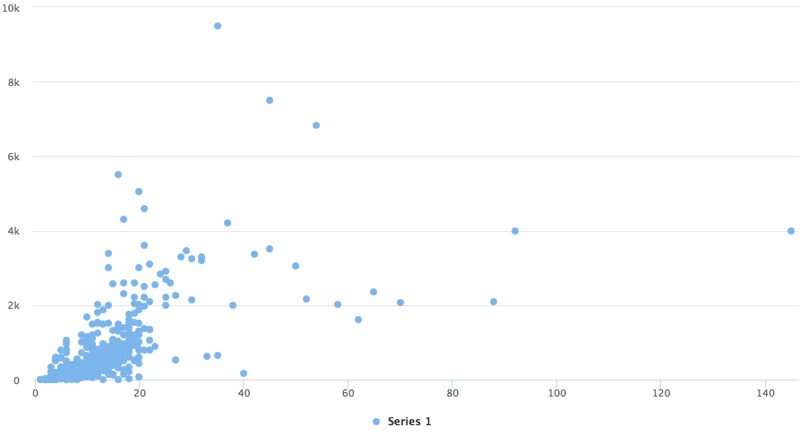
散点图

highchart()%>%
  hc_add_series(pokemon, "scatter", hcaes(x = height, y = weight))技术支持

与 ggplot2 的 geom_ 系列函数相比，hc_add_series 的主要区别在于：我们需要在每个函数中显式添加数据与映射，而在 ggplot2 中可以在某一层统一添加数据与映射，再继续添加多个基元（geoms）共享同一数据与映射。

下面用 ggplot2 包中的 diamond 数据集给出一个恰当示例。

data(diamonds, package = "ggplot2")

set.seed(123)
data <- sample_n(diamonds, 300)

modlss <- loess(price ~ carat, data = data)
fit <- arrange(augment(modlss), carat)

highchart() %>%
  hc_add_series(data, type = "scatter",
                hcaes(x = carat, y = price, size = depth, group = cut)) %>%
  hc_add_series(fit, type = "line", hcaes(x = carat, y = .fitted),
                name = "Fit", id = "fit") %>%
  hc_add_series(fit, type = "arearange",
                hcaes(x = carat, low = .fitted - 2*.se.fit,
                      high = .fitted + 2*.se.fit),
                linkedTo = "fit")技术支持

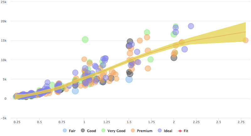
如示例所示，该图由三条系列构成：散点、折线与面积区间。

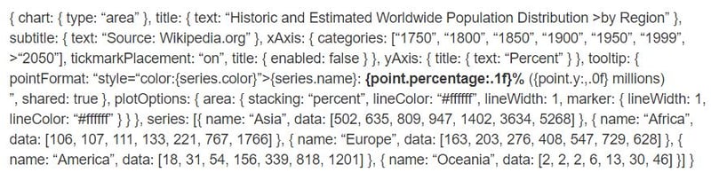
让我们用 hc_add_series 在 R 中复刻一段 highchart 的 JavaScript 开发。

highchart() %>%
  hc_chart(type = "area") %>%
  hc_title(text = "Historic and Estimated Worldwide Population Distribution by Region") %>%
  hc_subtitle(text = "Source: Wikipedia.org") %>%
  hc_xAxis(categories = c("1750", "1800", "1850", "1900", "1950", "1999", "2050"),
           tickmarkPlacement = "on",
           title = list(enabled = FALSE)) %>%
  hc_yAxis(title = list(text = "Percent")) %>%
  hc_tooltip(pointFormat = "<span style=\"color:{series.color}\">{series.name}</span>:
             <b>{point.percentage:.1f}%</b> ({point.y:,.0f} millions)<br/>",
             shared = TRUE) %>%
  hc_plotOptions(area = list(
     stacking = "percent",
     lineColor = "#ffffff",
     lineWidth = 1,
     marker = list(
       lineWidth = 1,
       lineColor = "#ffffff"
       ))
     ) %>%
  hc_add_series(name = "Asia", data = c(502, 635, 809, 947, 1402, 3634, 5268)) %>%
  hc_add_series(name = "Africa", data = c(106, 107, 111, 133, 221, 767, 1766)) %>%
  hc_add_series(name = "Europe", data = c(163, 203, 276, 408, 547, 729, 628)) %>%
  hc_add_series(name = "America", data = c(18, 31, 54, 156, 339, 818, 1201)) %>%
  hc_add_series(name = "Oceania", data = c(2, 2, 2, 6, 13, 30, 46))技术支持

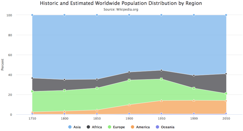
对比来看，您会发现每个 JavaScript 代码块都被转换成相互通过管道连接的 R 函数。我们可以看看一些参数，例如 hctooltip 的 pointFormat，其格式与 JavaScript 代码一致，详情可参见此处。

Highstocks

Highstocks 是用于金融与时间序列分析的图表，它与 quamtmod 库配合良好，绘制符号十分方便，然后您可以使用 hc_add_series 添加更多系列。

x <- getSymbols("GOOG", auto.assign = FALSE)

hchart(x)技术支持

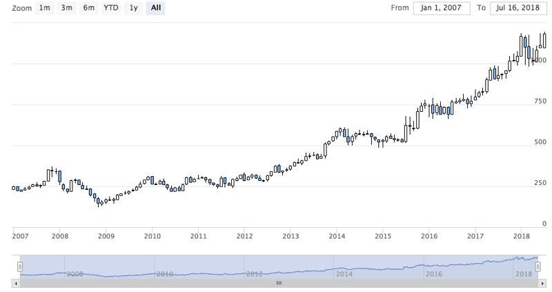
如图所示，我们无需添加额外代码，hchart 能很好地适配 xts 对象，提供数据的动态快照。您可以使用缩放功能将数据下钻为更小的区间，以便更好地分析。

我们来使用 hc_add_series。

y <- getSymbols("AMZN", auto.assign = FALSE)

highchart(type = "stock") %>%
  hc_add_series(x) %>%
  hc_add_series(y, type = "ohlc")技术支持

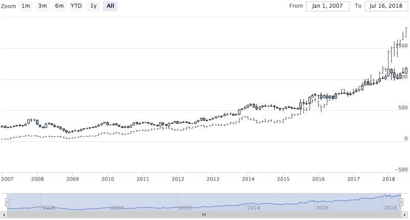
如您所见，这种可视化能高效地处理大体量数据。

不妨用不同的 xts 对象来尝试股票图。

Highmaps

用 highcharter 绘制地图的最简方式是使用 hcmap 函数。从 highmaps 的集合中选择一个 URL，并将该 URL 作为 hcmap 函数的地图参数。这会下载地图并使用信息创建一个对象，作为 mapdata 参数。

我们来绘制印度地图。

hcmap("https://code.highcharts.com/mapdata/countries/in/in-all.js")%>%
  hc_title(text = "India")技术支持

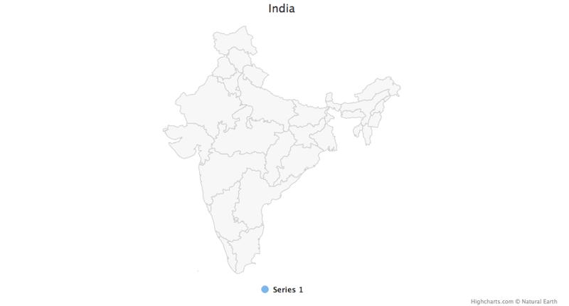
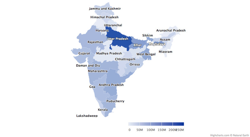
这只是一个底图，那么如何将其转换为分级着色地图呢？

从 Highcharts 地图集合下载的每个地图数据都有用于关联数据的键。这里有两个函数可以帮助了解地图中编码了哪些区域，以及如何将地图与数据关联：

download_map_data：从 Highcharts 集合下载 geojson 数据。
get_data_from_map：获取地图中各区域的属性，如地图数据中的键。

mapdata <- get_data_from_map(download_map_data("https://code.highcharts.com/mapdata/countries/in/in-all.js"))

glimpse(mapdata)技术支持

## Observations: 34
## Variables: 20
## $ `hc-group`    <chr> "admin1", "admin1", "admin1", "admin1", "admin1"...
## $ `hc-middle-x` <dbl> 0.65, 0.59, 0.50, 0.56, 0.46, 0.46, 0.51, 0.59, ...
## $ `hc-middle-y` <dbl> 0.81, 0.63, 0.74, 0.38, 0.64, 0.51, 0.34, 0.41, ...
## $ `hc-key`      <chr> "in-py", "in-ld", "in-wb", "in-or", "in-br", "in...
## $ `hc-a2`       <chr> "PY", "LD", "WB", "OR", "BR", "SK", "CT", "TN", ...
## $ labelrank     <chr> "2", "2", "2", "2", "2", "2", "2", "2", "2", "2"...
## $ hasc          <chr> "IN.PY", "IN.LD", "IN.WB", "IN.OR", "IN.BR", "IN...
## $ `alt-name`    <chr> "Pondicherry|Puduchcheri|PondichÃÂ©ry", "Ã\u008dl...
## $ `woe-id`      <chr> "20070459", "2345748", "2345761", "2345755", "23...
## $ fips          <chr> "IN22", "IN14", "IN28", "IN21", "IN34", "IN29", ...
## $ `postal-code` <chr> "PY", "LD", "WB", "OR", "BR", "SK", "CT", "TN", ...
## $ name          <chr> "Puducherry", "Lakshadweep", "West Bengal", "Ori...
## $ country       <chr> "India", "India", "India", "India", "India", "In...
## $ `type-en`     <chr> "Union Territory", "Union Territory", "State", "...
## $ region        <chr> "South", "South", "East", "East", "East", "East"...
## $ longitude     <chr> "79.7758", "72.7811", "87.7289", "84.4341", "85....
## $ `woe-name`    <chr> "Puducherry", "Lakshadweep", "West Bengal", "Ori...
## $ latitude      <chr> "10.9224", "11.2249", "23.0523", "20.625", "25.6...
## $ `woe-label`   <chr> "Puducherry, IN, India", "Lakshadweep, IN, India...
## $ type          <chr> "Union Territor", "Union Territor", "State", "St...技术支持

#population state wise
pop = as.data.frame(c(84673556, 1382611, 31169272, 103804637, 1055450, 25540196, 342853, 242911, 18980000, 1457723, 60383628, 25353081, 6864602,
12548926, 32966238, 61130704, 33387677, 64429, 72597565, 112372972, 2721756, 2964007, 1091014, 1980602, 41947358, 1244464,
27704236, 68621012, 607688, 72138958, 3671032, 207281477, 10116752,91347736))

state= mapdata%>%
  select(`hc-a2`)%>%
  arrange(`hc-a2`)

State_pop = as.data.frame(c(state, pop))
names(State_pop)= c("State", "Population")

hcmap("https://code.highcharts.com/mapdata/countries/in/in-all.js", data = State_pop, value = "Population",
      joinBy = c("hc-a2", "State"), name = "Fake data",
      dataLabels = list(enabled = TRUE, format = '{point.name}'),
      borderColor = "#FAFAFA", borderWidth = 0.1,
      tooltip = list(valueDecimals = 0))技术支持

试着在地图与分级着色图中搭配使用 hc_add_series 做些实验。更多细节与示例请访问这里。

插件

现在试试 highcharter 提供的一些插件功能，如分组、下钻、下载、打印数据，以及一些很棒的主题。

我们来对 mpg 数据集进行分组。为更佳的可视化，我们创建了一个列表，按制造商对数据进行分类。

data(mpg, package = "ggplot2")

mpgg <- mpg %>%
  filter(class %in% c("suv", "compact", "midsize")) %>%
  group_by(class, manufacturer) %>%
  summarize(count = n())

categories_grouped <- mpgg %>%
  group_by(name = class) %>%
  do(categories = .$manufacturer) %>%
  list_parse()

highchart() %>%
  hc_xAxis(categories = categories_grouped) %>%
  hc_add_series(data = mpgg, type = "bar", hcaes(y = count, color = manufacturer),
                showInLegend = FALSE)技术支持

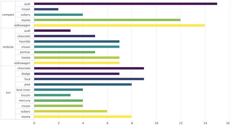
我们来创建一个可下钻到另一张图的图表，以便更好地分析。如果您理解 R 中的列表，这段代码会更容易看懂。

df <- data_frame(
  name = c("Animals", "Fruits", "Cars"),
  y = c(5, 2, 4),
  drilldown = tolower(name)
)


ds <- list_parse(df)
names(ds) <- NULL


hc <- highchart() %>%
  hc_chart(type = "column") %>%
  hc_title(text = "Basic drilldown") %>%
  hc_xAxis(type = "category") %>%
  hc_legend(enabled = FALSE) %>%
  hc_plotOptions(
    series = list(
      boderWidth = 0,
      dataLabels = list(enabled = TRUE)
    )
  ) %>%
  hc_add_series(
    name = "Things",
    colorByPoint = TRUE,
    data = ds
  )

dfan <- data_frame(
  name = c("Cats", "Dogs", "Cows", "Sheep", "Pigs"),
  value = c(4, 3, 1, 2, 1)
)

dffru <- data_frame(
  name = c("Apple", "Organes"),
  value = c(4, 2)
)

dfcar <- data_frame(
  name = c("Toyota", "Opel", "Volkswage"),
  value = c(4, 2, 2)
)

second_el_to_numeric <- function(ls){

  map(ls, function(x){
    x[[2]] <- as.numeric(x[[2]])
    x
  })

}

dsan <- second_el_to_numeric(list_parse2(dfan))

dsfru <- second_el_to_numeric(list_parse2(dffru))

dscar <- second_el_to_numeric(list_parse2(dfcar))

hc %>%
  hc_drilldown(
    allowPointDrilldown = TRUE,
    series = list(
      list(
        id = "animals",
        data = dsan
      ),
      list(
        id = "fruits",
        data = dsfru
      ),
      list(
        id = "cars",
        data = dscar
      )
    )
  )技术支持

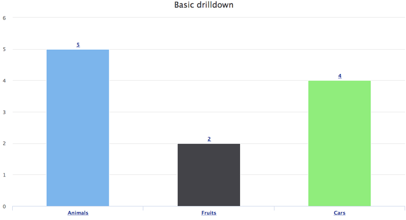
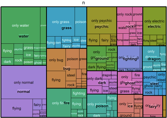
我们把下钻功能应用到其他图表上试试。

tm <- pokemon %>%
  mutate(type_2 = ifelse(is.na(type_2), paste("only", type_1), type_2),
         type_1 = type_1) %>%
  group_by(type_1, type_2) %>%
  summarise(n = n()) %>%
  ungroup() %>%
  treemap::treemap(index = c("type_1", "type_2"),
                   vSize = "n", vColor = "type_1")技术支持

tm$tm <- tm$tm %>%
  tbl_df() %>%
  left_join(pokemon %>% select(type_1, type_2, color_f) %>% distinct(), by = c("type_1", "type_2")) %>%
  left_join(pokemon %>% select(type_1, color_1) %>% distinct(), by = c("type_1")) %>%
  mutate(type_1 = paste0("Main ", type_1),
         color = ifelse(is.na(color_f), color_1, color_f))

highchart() %>%
  hc_add_series_treemap(tm, allowDrillToNode = TRUE,
                        layoutAlgorithm = "squarified")技术支持

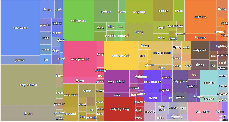
我们再添加数据导出功能。

pokemon%>%
  count(type_1)%>%
  arrange(n)%>%
  hchart(type = "bar", hcaes(x = type_1, y = n, color = type_1))%>%
  hc_exporting(enabled = TRUE)技术支持

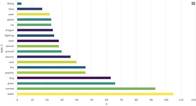最后，我们加上一些主题。

pokemon%>%
  count(type_1)%>%
  arrange(n)%>%
  hchart(type = "bar", hcaes(x = type_1, y = n, color = type_1))%>%
  hc_exporting(enabled = TRUE)%>%
hc_add_theme(hc_theme_chalk())技术支持

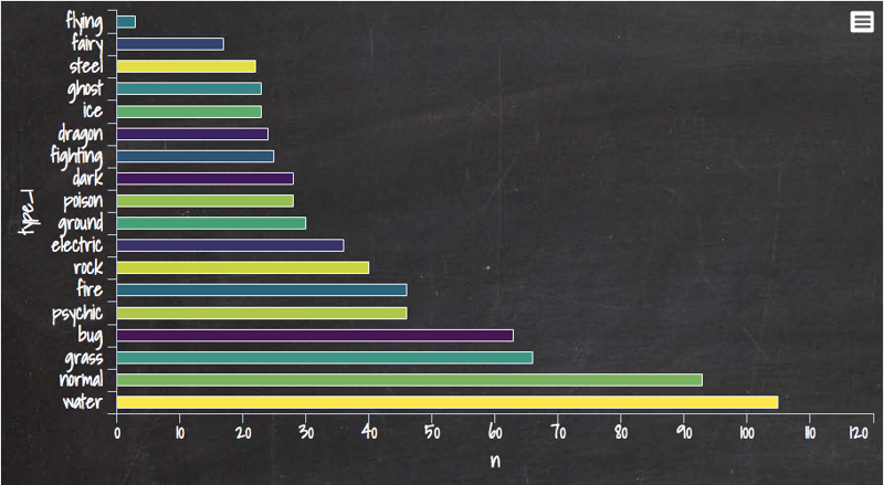
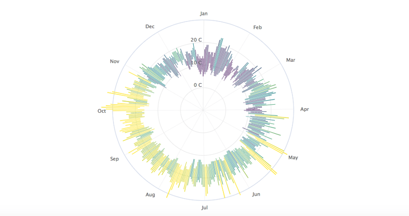
您可以从这里学到很多内容，它是 Highcharter 的完整库文档。我还分享一张我最喜欢的基于天气数据集创建的图表，其中使用了一个很有意思的参数 polar：将其设为 TRUE 后，整个呈现方式都变了。

data("weather")

x <- c("Min", "Mean", "Max")
y <- sprintf("{point.%s}", c("min_temperaturec", "mean_temperaturec", "max_temperaturec"))
tltip <- tooltip_table(x, y)

hchart(weather, type = "columnrange",
       hcaes(x = date, low = min_temperaturec, high = max_temperaturec,
             color = mean_temperaturec)) %>%
  hc_chart(polar = TRUE) %>%
  hc_yAxis( max = 30, min = -10, labels = list(format = "{value} C"),
            showFirstLabel = FALSE) %>%
  hc_xAxis(
    title = list(text = ""), gridLineWidth = 0.5,
    labels = list(format = "{value: %b}")) %>%
  hc_tooltip(useHTML = TRUE, pointFormat = tltip,
             headerFormat = as.character(tags$small("{point.x:%d %B, %Y}")))技术支持

如果您想进一步学习 R 中的数据可视化，请参加 DataCamp 的Data Visualization with ggplot2 (Part 1)课程，并查看我们的R 公式教程。

主题

数据可视化数据科学 R

主题

技术

使用 R 的 Highcharter 进行数据可视化

使用 AI 探索

使用 hchart 函数创建一些基础图表

矩形树图

散点图

Highstocks

Highmaps

插件

主题

了解更多 R 与数据可视化

使用 ggplot2 进行数据可视化入门

R 中的 plotly 交互式数据可视化

R 中的可视化最佳实践

主题

技术

了解更多 R 与数据可视化

使用 ggplot2 进行数据可视化入门

R 中的 plotly 交互式数据可视化

R 中的可视化最佳实践