Have this cheat sheet at your fingertips
Download PDFDefinitions
- The majority of data analysis in R is performed in data frames. These are rectangular datasets consisting of rows and columns.
- An observation contains all the values or variables related to a single instance of the objects being analyzed. For example, in a dataset of movies, each movie would be an observation.
- A variable is an attribute for the object, across all the observations. For example, the release dates for all the movies.
- Tidy data provides a standard way to organize data. Having a consistent shape for datasets enables you to worry less about data structures and more on getting useful results. The principles of tidy data are:
-
- Every column is a variable.
- Every row is an observation.
- Every cell is a single value.
Helpful syntax before getting started
Installing and loading tidyr
# Install tidyr through tidyverse
install.packages("tidyverse")

# Install it directly
install.packages("tidyr")

# Load tidyr into R
library(tidyr)
The %>% Operator
%>% is a special operator in R found in the magrittr and tidyr packages. %>% lets you pass objects to functions elegantly, and helps you make your code more readable. The following two lines of code are equivalent.
# Without the %>% operator
second_function(first_function(dataset, arg1, arg2), arg3)

# With the %>% operator
dataset %>% some_function(arg1, arg2) %>% second_function(arg3)
Datasets used throughout this cheat sheet
Throughout this cheat sheet we will use a dataset of the top grossing movies of all time, stored as movies.
|
title |
release_year |
release_month |
release_day |
directors |
box_office_busd |
|
Avatar |
2009 |
12 |
18 |
James Cameron |
2.922 |
|
Avengers: Endgame |
2019 |
4 |
22 |
Anthony Russo,Joe Russo |
2.798 |
|
Titanic |
1997 |
11 |
01 |
James Cameron |
2.202 |
|
Star Wars Ep. VII: The Force Awakens |
2015 |
12 |
14 |
J. J. Abrams |
2.068 |
|
Avengers: Infinity War |
2018 |
4 |
23 |
Anthony Russo,Joe Russo |
2.048 |
The second dataset involves an experiment with the number of unpopped kernels in bags of popcorn, adapted from the Popcorn dataset in the Stat2Data package.
|
brand |
trial_1 |
trial_2 |
trial_3 |
trial_4 |
trial_5 |
trial_6 |
|
Orville |
26 |
35 |
18 |
14 |
8 |
6 |
|
Seaway |
47 |
47 |
14 |
34 |
21 |
37 |
The third dataset is JSON data about music containing nested elements. The JSON is parsed into nested lists using parse_json() from the jsonlite package.
|
artist |
singles |
|
|
Bad Bunny |
title |
tracks |
|
Gato de Noche |
Gato de Noche, Ñengo Flow |
|
|
La Jumpa |
La Jumpa, Arcángel |
|
|
Drake |
title |
tracks |
|
Scary Hours 2 |
What's Next, Wants and Needs, Lemon Pepper Freestyle, NA, Lil Baby, Rick Ross |
|
The fourth dataset is a synthetic dataset containing attributes of people. sex is a character vector, and hair_color is a factor.
|
sex |
hair_color |
height_cm |
weight_kg |
|
female |
brown |
166 |
72 |
|
male |
blonde |
184 |
|
|
female |
black |
153 |
|
|
male |
black |
192 |
93 |
Uniting and separating columns
# Combine several columns into a single vector column with unite()
movies %>%
  unite(release_date, c(release_year, release_month, release_day), sep = "-")
# Split a single vector column into several columns with separate()
movies %>%
separate(directors, into = c("director1", "director2"), sep=",", fill = "right")# Split a single column into several rows with separate_rows()
movies %>%
separate_rows(directors, sep=",")Packing and unpacking columns
# Combine several columns into a data frame column with pack()
movies_packed <- movies %>%
  pack(release_date = c(release_year, release_month, release_day))
# The release date column is a data frame with 5 rows, 3 columns
# Split a single data frame column into several columns with unpack()
movies_packed %>%
unpack(release_date)
# release_date column replaced with release_year/release_month/release_day columnsPivoting
# Move side-by-side columns to consecutive rows with pivot_longer()
popcorn_long <- popcorn %>%
  pivot_longer(trial_1:trial_6, names_to = "trial", values_to = "n_unpopped")

# "brand" columns contains "Orville" and "Seaway"

# "trial" column contains "trial_1" to "trial_6"

# "n_unpopped" column contains the numbers
# Move values in different rows to columns with pivot_wider()
popcorn_long %>%
pivot_wider(brand, names_from = "trial", values_from = "n_unpopped")
# Same contents and shape as popcorn datasetNesting and unnesting
# Expand nested data frame columns with unnest_longer()
# Vectors inside the nested data are given their own row
# The number of columns remains unchanged
music %>%
  unnest_longer(singles)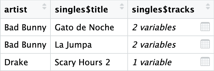
# Expand nested data frame columns with unnest_wider()
# Top-level elements inside the nested data are given their own column
# The number of rows remains unchanged
music %>%
  unnest_wider(singles)
# Expand selected nested data frame columns with hoist()
# Replacement for unnest_wider() %>% select()
music %>%
  hoist(singles, single_titles = "title")
# Expand nested data frame columns with unnest_longer()
# Every top-level element of the nested data gets its own column in the result
# Vectors inside the nested data are given their own row
music_unnested <- music %>%
  unnest(singles)
# Roughly equivalent to music %>% unnest_longer(singles) %>% unnest_wider(singles)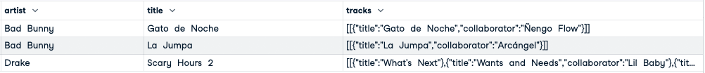
# Summarize parts of a data frame as a list of dataframes with nest()
music_unnested %>%
  nest(singles = c(title, tracks))
Dealing with missing data
# Drop rows containing any missing values in the specified columns with drop_na()
people %>%
  drop_na(weight_kg)
# Replace missing values with a default value with replace_na()
people %>%
replace_na(list(weight_kg = 100))Creating grids
# Get all combinations of input values with expand_grid()
expand_grid(
  sex = c("male", "female", "female"),
  hair_color = c("red", "brown", "blonde", "black", "red")
)

# 2 column data frame with rows like "male", "red".
# Get all combinations of input values, deduplicating and sorting with crossing()
crossing(
sex = c("male", "female", "female"),
hair_color = c("red", "brown", "blonde", "black", "red")
)
# Same as expand_grid() but "red" rows only appear once and order is alphabetical# Get all combinations of values in data frame columns with expand()
# All factor levels included, even if they don't appear in data
people %>%
expand(sex, hair_color)
# Equivalent to expand_grid(unique(people$sex), levels(people$hair_color))# Get all combinations of values that exist in data frame columns with expand() + nesting()
people %>%
expand(nesting(sex, hair_color))
# As previous, but filtered to rows that exist in people dataset# Expand the data frame, then full join to itself with complete()
people %>%
complete(sex, hair_color)
# Same output as expand, with additional height_cm and weight_kg columns# Fill in sequence of numeric or datetime columns with expand() + full_seq()
people %>%
expand(height_cm_expanded = full_seq(height_cm, 1))
# 1 column data frame with height_cm_expanded values
# from min height_cm to max height_cm in steps of 1