Curso
No matter how sophisticated our analytics or predictive algorithms are, the quality of output is dependent on the data input. In other words, 'garbage in, garbage out.'
Since data underpins all of these processes, it is important to spend ample time ensuring that data is properly refined.
Data cleaning is a foundational process in the data science lifecycle, and its role cannot be overemphasized when trying to uncover insights and generate reliable answers. More often than not, data will always be dirty in the real world, and data cleaning cannot be completely avoided.
In this article, we will cover some important ideas, like how to handle missing values, duplicates, and outliers. For a more comprehensive set of instructions, make sure to take our Cleaning Data in Python or Cleaning Data in R course.
What Causes Unclean Data?
Simply put, data cleaning (or cleansing) is a process required to prepare for data analysis. This can involve finding and removing duplicates and incomplete records, and modifying data to rectify inaccurate records.
Unclean or dirty data has always been a problem, yet we have seen an exponential rise in data generation over the last decade. In 2020 alone, the world generated more than 64 zettabytes of data, an equivalent of 6.4 trillion gigabytes. While less than 2% of all this data is retained, it still undoubtedly compounds the already existing common problem of "dirty data." Before data cleaning can properly be done, it is important to understand how it got dirty in the first place. This can arise from common sources such as:
- Human error during data entry, recording, or encoding
- A faulty sensory device, as is the case in the internet of things (IoT)
- Corruption is a result of hardware or software damage.
Being aware of the root cause of the dirty data we intend to clean lays a good foundation for imposing data quality criteria that allow classifying the different problems associated with our dataset.
Why is Data Cleaning so Important?
The process of data cleaning is important as it helps to create a template for cleaning an organization's data. As mentioned earlier, any data analytics or data science process is garbage in, garbage out. When neglected, the result of it is costly, erroneous analytical results, both in terms of time and money, as well as other committed resources.
What is Data Quality?
Data quality is the qualitative and or quantitative measure of how well our data suits the purpose it is required to serve. These measures are practical templates we can use to assess how suitable the data provided is for our desired purposes. Consider these data quality measures as metrical tests our data must pass to deem it fit for data science processes.
Criteria for data quality
- Accuracy: A simple question we can ask to verify accuracy is - is the information contained in the data provisioned correctly in every detail? With data, we are trying to approximate patterns in the real world; accuracy helps define how true these approximations are.
- Relevance: Is this information impactful to what our desired end goal is?
- Consistency: Is the source of this data verified and can the information contained there be trusted? For example, having a customer who is age 15 but marital status is indicated to be married.
- Completeness: Is the data provisioned and comprehensive enough for the desired end goal? This is a common problem associated with missing data and one way to resolve this is by investigating the data source.
- Uniformity: Let's assume we have a sales column but not all transactions are made in the same currency. It becomes imperative to convert all the sales values into a single currency and that is what uniformity is about; ensuring that data measures are specified using the same units of measure in all systems.
Data cleaning vs. data transformation
It is important to mark a distinction between data cleaning and data transformation. Data transformation is a set of processes that can help us extract more insights from the data provided. These processes will typically change the raw format of the data into another format, a few examples include:
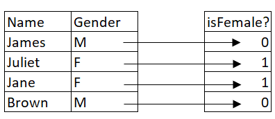
- Encoding: This is a process of converting categorical values into binary values which can then be used in computations for machine learning. The figure shows what the gender column would look like if it were encoded. While it still carries the same information, it has been transformed into a different format.
- Data binning: Also referred to as bucketing, this process helps to reduce the effect/size of minor observations. It entails grouping continuous values into bins (or categories).

- Scaling: This is a common technique in machine learning to help standardize values of different scales into a fixed range.
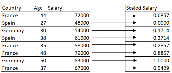
Notice how in most data transformation processes, the original representation of the data is altered. While it is still the same data, certain techniques have been introduced to transform it into a format usable for machine learning or some other purpose.
How Data Cleaning is Done
It is important to have a set of guidelines to achieve high-quality data. These guidelines can be referred to as a data cleaning workflow. They help us take into account all the processes necessary for data cleaning. The processes included in this workflow are:
- Data exploration
- Data cleaning
- Data verification
- Data cleaning reporting Some of these processes will also be demonstrated in Python
Data exploration
Data exploration is all about understanding the data via a deep exploration of the variables present in the data. It requires a number of visual and aggregation techniques to properly uncover underlying issues with the data. For proper exploration, here are a few points to note:
Data Context
Before we can clean any data, we must understand the context of the data. Data context is the source of all entities contained in data. It captures the set of circumstances that surround how data is collected, and how it is collected gives insights into how it can be used and what it can be used for.
This serves as a guiding light into what is acceptable in cleaning (and analysis) so we can derive the right insights from such data. Once we have a clear knowledge of how the data is/was collected, we then need to explore such data.
Exploratory Data Analysis
Exploratory data analysis refers to the critical process of performing initial investigations on data so as to discover patterns, spot anomalies, test hypotheses, and check assumptions with the help of summary statistics and graphical representations. There is no discovery without exploration. If we don't explore our data, it's difficult to discover the various issues existing within the data.
For example, we have a dataset provided for us here. The Department of Finance's Rolling Sales files list properties that sold in the last twelve-month period in New York City for tax classes 1, 2, and 4. We will download and read the Bronx data provided.
#pandas
import pandas as pd
import seaborn as sns
import matplotlib.pyplot as plt

#read excel file
df = pd.read_excel("rollingsales_bronx.xls")

#preview data
df.head()
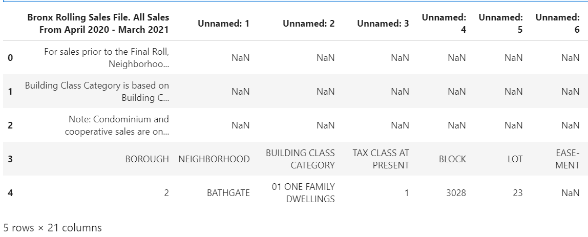
The notable issues with this data frame include:
- unnamed columns
- missing values in the first three rows
However, exploring the actual data in excel reveals that the actual table in the workbook doesn't start until the 4th row. Therefore, reading the data again but setting a few parameters allows us to indicate which rows to skip and which row to make into the header:
#we read the data in again but skill 3 rows this time
df = pd.read_excel("rollingsales_bronx.xls", skiprows = 4, header = [0])

df.head()
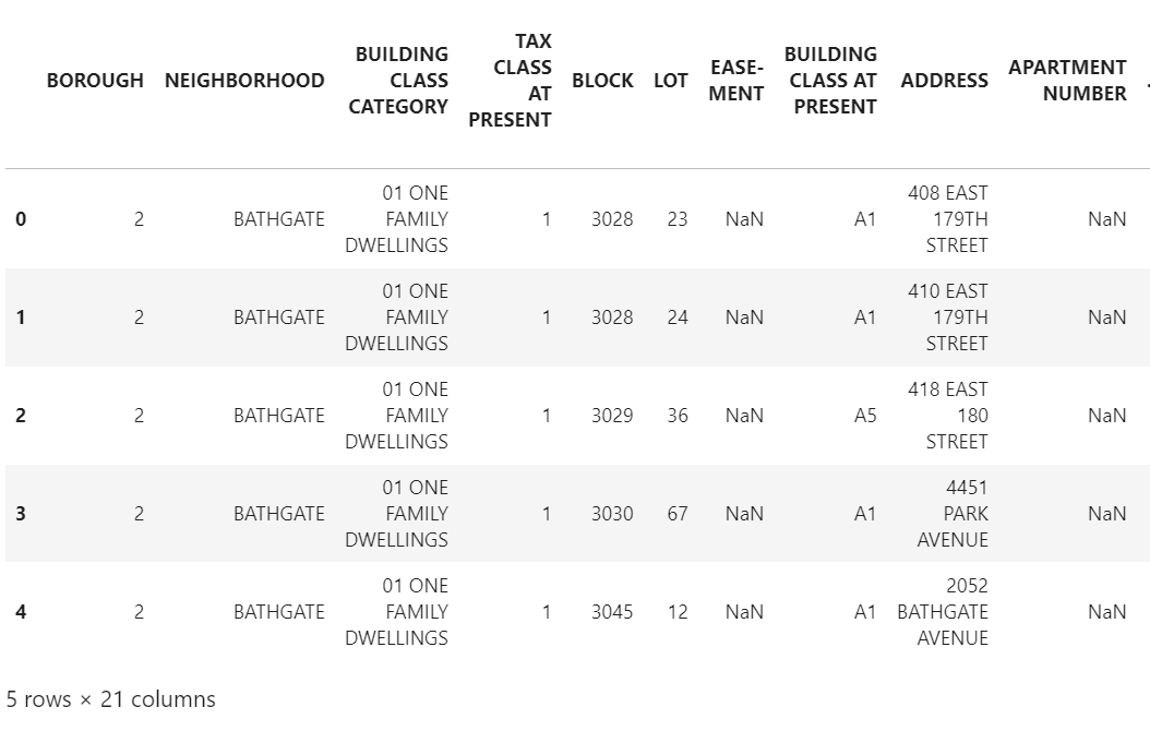
There is a significant change in how data is now displayed. While we could have cleaned the first import, data exploration has helped us save ample time with just a few modifications to our data import function in Python.
Data exploration is like walking into a crime scene as an investigative agent, where we passively observe all things out of place and data cleaning is the active process of solving the actual crime.
Data cleaning
Data exploration will typically go hand in hand with data cleaning processes. Once we uncover issues with our data using visual, aggregation, or statistical means, we need to fix them. In this phase, data will either be removed, corrected, or imputed.
Inconsistent Records
A typical example of inconsistent records is a form where individuals are required to enter their gender. We can have different formats representing the same thing e.g 'M', 'm', 'Male', or 'MALE', and did we sell 'aples', 'apples', or 'APPLES' this month. The best way to spot them can be via a frequency chart or making a distinct display of all values in the column. Some operations on inconsistent records will include but are not limited to:
- Converting strings to lower or proper case
- Removing white spaces
- Renaming column names
Python example: Using the dataset imported earlier under data exploration, notice how the column names are inconsistently written:

While this doesn't seem to be a big deal, it is important to make column names consistently accessible. For example, EASE-MENT has a hyphen (-) between each word, while the rest just have spaces.
Part of data cleaning is ensuring consistency. Let us attempt to fix this in two steps:
- Replace spaces between words with an underscore
- Convert to proper case
# Extract columns
cols = df.columns

# Create empty list for new column names
new_cols = []

# Iterate over each column name to fix issues
for column in cols:
    # Convert column name to title case
    proper_cols = column.title()
    # Replace spaces and hyphens with underscores
    proper_cols_hyphen = proper_cols.replace(" ", "_")
    clean_col = proper_cols_hyphen.replace("-", "_")
    # Append the cleaned column name to the list
    new_cols.append(clean_col)

# Display the transformed column names
new_cols

# Replace existing columns in the dataframe with the cleaned list
df.columns = new_cols

# Preview the updated dataframe
df.head()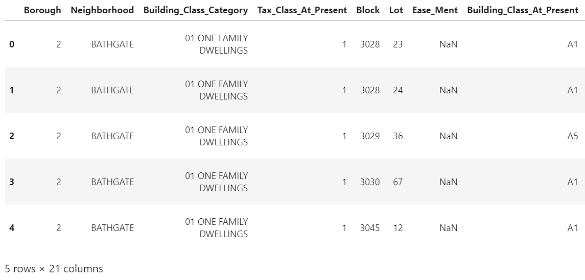
Data types and type conversion
The data type is simply how data is represented, which tells the compiler how the data is to be used. How data is represented determines the kind of operations possible with such data. Let us preview the data types in each column of our dataframe from the Bronx data.
#data types
df.dtypes
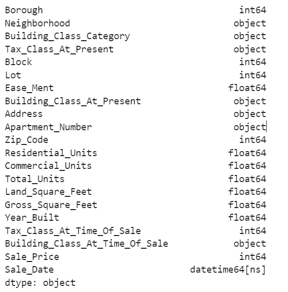
NB: Consider how we are now able to easily pick column names using the dot method (df.Year_Built).
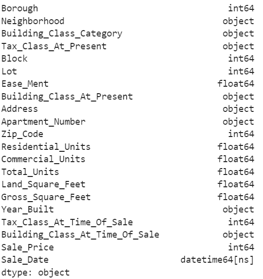
All data types appear in order except the Year_Built column, which should be categorical. While this has no major significance, when we aggregate these columns Year_Built will likely be included.
#Fix Year_Built column
df.Year_Built = df.Year_Built.astype("str")

#Check
df.dtypes
Missing data
There are times when there are observations (rows) with missing data and sometimes you can have entire columns with completely missing values. So what do we do in instances like this? Do we ignore it? This can be likened to a leaking roof and when it rains, it leaks.
Missing values have different representations across different tools. These representations include NULL, empty strings, NaN, NA, #NA, etc. Data context is important in dealing with missing data, and understanding why data is missing is crucial. There are two primary methods for dealing with missing data:
- Removal of data
- Imputation of data
Before any decision can be made on what method will be used, one must first examine the patterns of missing values across columns. We will use visual and descriptive techniques to assess these.
#extract the column names
cols = df.columns

#plot a heatmap of missing values with seaborn
plt.figure(figsize = (10,5))
sns.heatmap(df[cols].isnull())
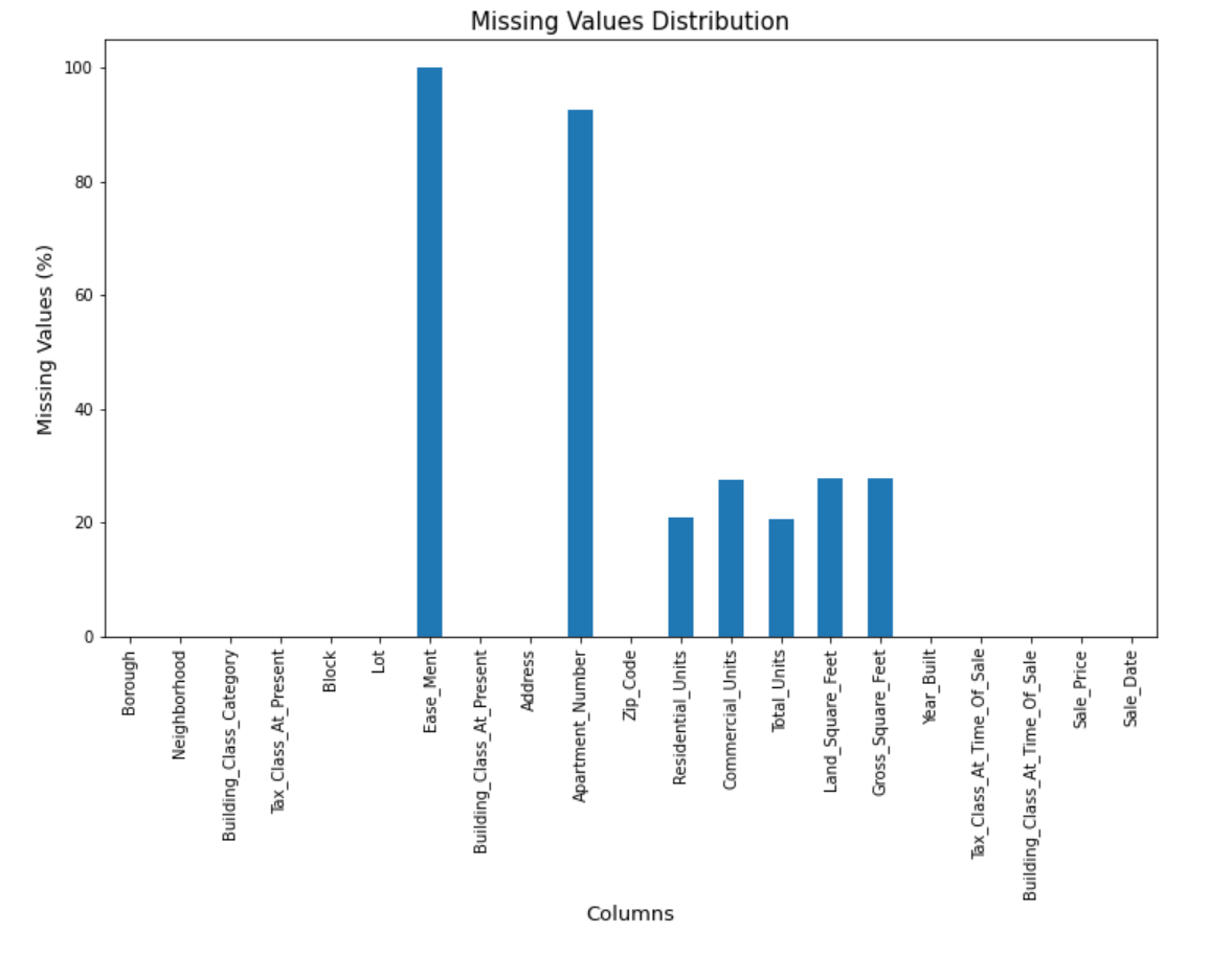
The plot visually shows that:
- All values in Ease_ment and almost all values in Apartment_Number are missing
- The Units and Square_Feet-related columns have missing values spread out For much larger datasets, this plot might not be ideal. Another way to handle this is to examine how significant these missing values are compared to the actual data size.
#Get the percentage of missing values in each column
missing_pct = round(df.isnull().sum()/len(df) * 100, 1)
print(missing_pct)
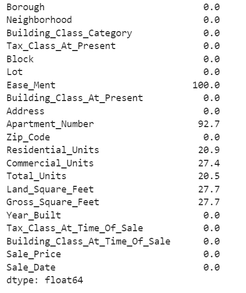
We will drop columns Ease_Ment and Apartment_Number and then replace the missing values in the remaining columns.
#columns with more than 30% missing values
drop_cols = missing_pct[missing_pct > 30].index
#We can drop these columns with greater than 30 percent missing values
df_new = df.drop(columns = drop_cols)

#Extract columns with mising values between 1 and 30%
replace_cols = missing_pct[(missing_pct > 0) & (missing_pct < 30)].index

#Iterate to replace missing values
for col in replace_cols:
    #if column is year built we replace with median otherwise the mean
    if col == "Year_Built":
        df_new.fillna(df_new[col].median(), inplace = True)
    else:
        mean_value = df_new[col].mean()
        df_new.fillna(mean_value, inplace = True)
df_new.isnull().sum() #preview for missing values
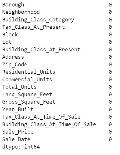
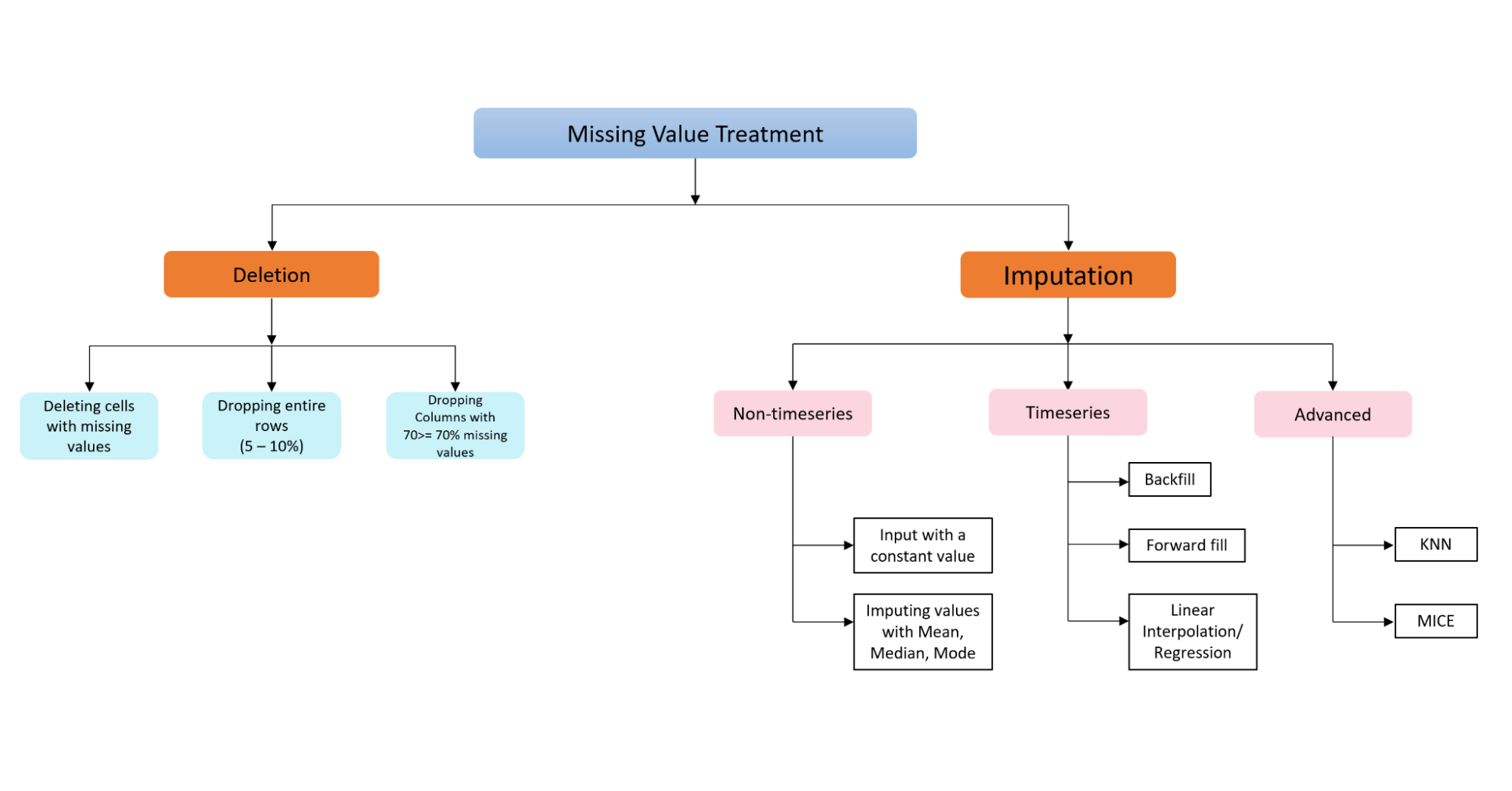
Of course, there's more to dealing with missing values, such as is covered in this Datacamp course on Dealing with Missing Values in Python. Different datasets, types, and structures have different needs, and therefore, dealing with missing values is not a straight, clear-cut process for all kinds of datasets. The image below shows different scenarios to apply either a deletion technique or an imputation technique.
Duplicates
We must ensure that we have a single source of truth for each observation. There are scenarios where we have multiple observations about a single customer, either because there is a double form submission by the user, or errors were made during data entry. Regardless of how this comes about, we need to develop a single, complete version of the truth. This will help businesses ensure that:
- Time and money is not wasted targeting the same customer twice
- A trusted and complete version of the truth is developed, and reliable business decisions can be made based on the analysis results.
Outliers
Outliers are extreme data points. They are usually very low or very high values that do not conform to the rest of the pattern in the data, for example:
- A customer who is 200 years of age
- A sensor reading of 40° Celsius in the Antarctica region
Identifying Outliers There are different techniques to identify outliers either through visual means or statistical techniques
-
Sorting the dataset: By simply sorting the data, one can easily spot outliers within the dataset or variables of interest. However, this technique fails on large datasets and can be difficult to preview all values at a glance.
-
Visualization: Using Visual techniques such as boxplots, histograms and scatterplots can make it easy to detect outliers.
-
Using Z-scores: This is a statistical technique to quantify the unusualness of an observed value assuming the data follows a normal distribution. It is the number of standard deviations by which observed values fall above or below a mean value.
Outlier Treatment Process Outlier treatment serves as a process of removing or replacing outliers represented in our data:
- Remove outliers from the data: This can involve removing values that lie at the lower or upper X_percentile of your data. The following are certain scenarios where outliers can be removed:
- When it is obvious that the data is incorrectly measured. As mentioned earlier, an active customer who is 200 years is not a valid input, a typical example of an outlier that should be removed.
-
If the outlier doesn't change the results of your analysis, you may drop this outlier. This can also be considered when the number of outliers in the dataset is not much in comparison to the overall data.
-
Replace outliers: This involves replacing these extreme values with the mean, median or modal values. If the number of outliers is of considerable size in comparison to the actual data, then removing outliers will fail. Note: Mean values are susceptible to outliers. It is therefore advisable to consider the median or modal value for replacement.
Data Verification
Once data cleaning is done, it is important to again reassess the quality of the data via the data exploration method. This is to verify the correctness and completeness of the data cleaning process, partly to ensure we didn't omit a step, and also to ensure we are in line with the data's context.
Data cleaning, reporting, and automation
Reporting involves documenting the health of the data post-cleaning, as well as documenting the processes involved in the cleaning process. Reporting ensures that there is a guide for future similar data cleaning needs (reproducibility), so that this process can be automated when needed again.
Automation is all about ensuring data cleaning is reproducible. Much of the data cleaning process consists of reusable scripts as such can be reused with just a few changes, should the need arise.
Conclusion
We have discussed data cleaning in-depth and all the components you need to take into account for a successful data cleaning project. It is a time-consuming phase upon which data professionals spend an estimated 60% of the entire data science project. It is a foundation that will single-handedly determine the outcome of a data science project. Different data from different sources have varying needs and you will need to adapt the processes accordingly to suit your use case.
Resource:
- The images associated with data transformation are snipped from an excel workbook found here
- The Python notebook is available on DataCamp workspace
