
Programa
Engenheiro de dados Em Python
40 h
Binary search trees (BSTs) are a type of binary tree data structure that organizes data using a specific ordering. Each node contains a value and has links to up to two other nodes: the left and right children. In a BST, the rule is that the value of the left child node must be less than its parent node's value, and the value of the right child node must be greater.
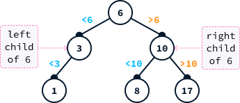
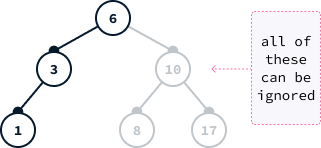
BSTs can be highly efficient for finding specific values because they allow us to eliminate large portions of the tree during the search process. For instance, if we're searching for the value one in the tree above, we can disregard all nodes to the right of six. This is because the order property guarantees that all those values are greater than six.
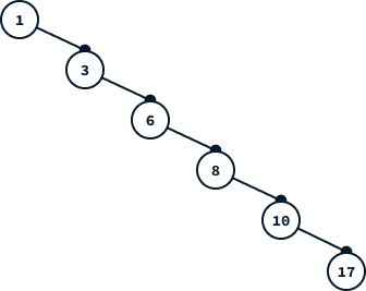
Ideally, each node should split the data in half, so that half of the values are eliminated at each step down the tree. This leads to extremely fast lookups. However, depending on the order of insertion, it's possible to end up with an unbalanced tree that does not effectively split the data. For instance, inserting values from smallest to largest will result in a linear tree, which performs no better than a list.
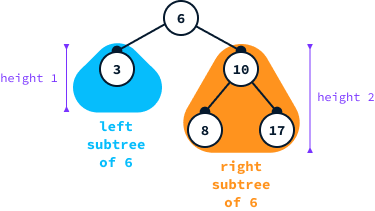
An AVL tree is a binary search tree with the following added property:
For each node, the height of the left and right subtrees differ by at most one.
Breaking down this definition, the left subtree of a node includes all nodes to its left, while the right subtree comprises all nodes to its right. The height of a tree is defined as the length of the longest path from the root node (the topmost node) to any of its descendant leaves (nodes without children).
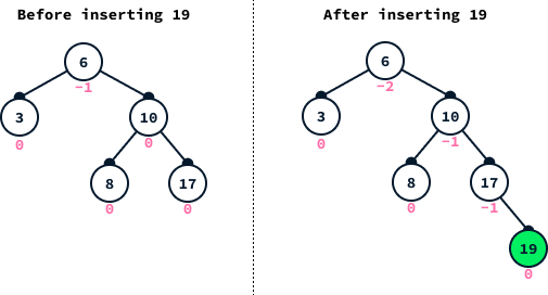
The balance factor of a node is calculated as the height difference between its left subtree and its right subtree:
balance(N) = height(left subtree of N) - height(right subtree of N)
For example, balance(6) = 1 - 3 = -2.
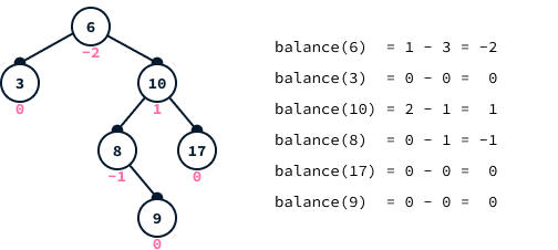
In the diagram, node 6 exhibits a balance factor equal to -2, indicating that the tree does not conform to AVL tree criteria. For a tree to be classified as an AVL tree, the balance factor of each node must be -1, 0, or 1.
The efficiency of queries in a binary search tree depends on the tree's height. In the worst-case scenario, the number of nodes that need to be examined is equal to the height of the tree. A key issue with BSTs is that the tree's height can match the number of nodes, meaning a query might necessitate inspecting every single node.
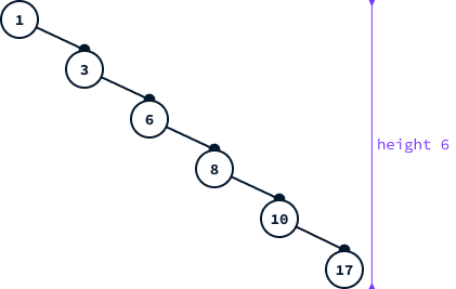
Let M(h) denote the minimum number of nodes required to add to a binary search tree to achieve a height of h. For simple BSTs, we have observed that M(h) = h, meaning we can attain a height of h using just h nodes. This implies that the height of a BST can increase linearly with the number of nodes, leading to a query time that is proportional to the size of the dataset.
Let's consider the minimum number of nodes, M(h), required to create an AVL tree with a height of h. Since it is an AVL tree, it is important to note that the balance factor of every node can only be -1, 0, or 1.
However, given our assumption that the tree has the fewest nodes possible to achieve a height of h, the root cannot have a balance of 0. If it did, we could remove a node from the left or the right side to achieve a balance of either -1 or 1, which would still result in a valid AVL tree.
Let's assume the root's balance is 1 (the reasoning would be the same if the balance were -1). This implies that the tree is structured as follows:
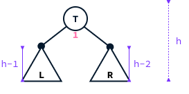
On the other hand, both the left and right subtrees must also be AVL trees, each with the minimum number of nodes required for their respective heights (otherwise, it would be possible to remove additional nodes). The total number of nodes in the tree equals 1 (for the root) plus the number of nodes in the left subtree plus the number of nodes in the right subtree.
M(h) = 1 + (nodes in L) + (nodes in R) = 1 + M(h - 1) + M(h - 2)
As the height grows, we need to add more nodes to reach that height. Therefore:
M(h - 1) > M(h - 2)
Combining the two, we can say that:
M(h) = 1 + M(h - 1) + M(h - 2) > 1 + 2 × M(h - 2) > 2 × M(h - 2)
We can apply this h/2 times until we each either M(1) = 1 or M(2) = 2:
M(h) > 2 × M(h - 2) > 2 × 2 × M(h - 4) > 2 × 2 × 2 × M(h - 6) > … > 2(h/2)
For clarity, the following image shows the specific examples when h = 7 and h = 6:
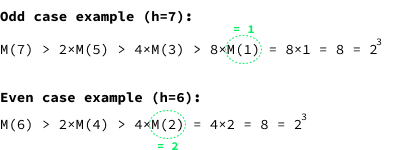
We conclude that the minimum number of nodes in an AVL tree of height h is at least 2(h/2):
M(h) > 2(h/2)
By applying the logarithm base two to both sides, we obtain:
log2(M(h)) > log2(2(h/2)) = h/2
Consequently, by multiplying both sides by two, we deduce that the height is at most twice the base-2 logarithm of the number of nodes:
2 × log2(M(h)) > h
We have demonstrated that:
The height of an AVL tree containing N nodes is at most 2 × log2(N).
This indicates that queries within an AVL tree only necessitate examining a small segment of the dataset. For instance, given one billion entries, the logarithm equates to approximately 30, meaning that even with one billion data points, it's necessary to inspect only around 60 data points to find a specific entry. This represents a significant enhancement compared to BSTs, which, in the worst-case scenario, would require inspecting the entire one billion data points.
For a more in-depth understanding of algorithmic time complexity and the difference between linear time complexity and logarithmic complexity, check out this blog post on Big-O Notation and Time Complexity.
AVL trees guarantee fast queries by enforcing that the balance of each node is either -1, 0, or 1. To ensure that the balance of each node is maintained, we need to rebalance the tree after inserting a new value.
Insertion in binary search trees works by following the path from the root down the tree. We go left whenever the value we want to insert is smaller and right otherwise.
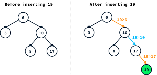
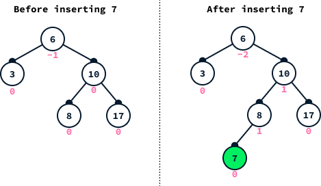
An insertion increases the height by at most one. So, if the balance property isn’t respected after insertion, it means that there was either a node with balance -1, which now has balance -2, or a node with balance 1, which now has balance 2. The first case is what happens in the above example.
To restore balance, we rely on tree rotations. A left rotation on node A restructures the tree by rotating A to the left, as shown below:
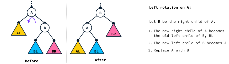
On the diagram:
BL represents the left subtree of BBR is the right subtreeAL is the left subtree of ANote that after rotation, the node order is still valid:
A is smaller than B because B was its right child.BL are larger than A because they were on the right of A.AL are smaller than B because they are smaller than A.A right rotation works in the same symmetric way by rotating A to the right.
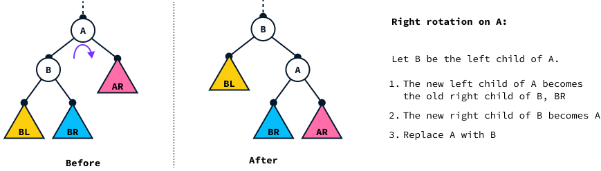
Let’s see a concrete example by fixing the imbalance of the tree after inserting 19 using a left rotation on node 6.
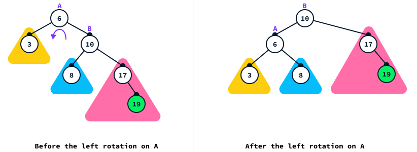
After insertion, we’ll fix the imbalance by rotating a node with a balance of -2 or 2. In this case, the balance factor of node 6 was -2, meaning that the tree was leaning to the right, so we applied a left rotation (in the direction opposite of the imbalance). If, instead, the balance is equal to 2, then a right rotation is used instead.
In the previous example, the tree was fully leaning to the right, so a single left rotation was enough to restore balance. However, in some cases, we have a zig-zag type of imbalance where the tree leans to one side, but the subtree leans to the opposite side. To see this, let’s go back to the original tree before we inserted 19 and insert 7 instead:
In this case, the tree is still leaning to the right, but the subtree rooted at 10 is leaning to the left. In this case, we first need to rotate node 10 to the right:
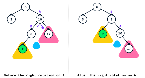
Note that node B doesn’t have the right child. We still display it in blue in the diagram to make it easier to visualize.
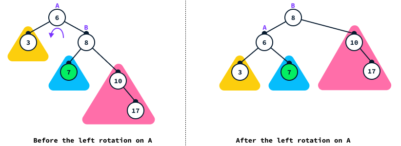
After performing the right rotation, we fall back into the previous case where a left rotation on 6 will restore balance:
Let’s start with the node implementation.
Each node of the tree has five attributes:
self.value)self.parent)self.left)self.right)self.height)class Node:
def __init__(self, value, parent = None):
self.value = value
self.parent = parent
self.left = None
self.right = None
self.height = 1We employ the value None to represent missing nodes. The default height is set to 1 because a tree consisting of a single node has a height of 1.
To facilitate the tree implementation, we introduce several methods to the Node class.
# Inside the Node class
  def left_height(self):
    # Get the heigth of the left subtree
    return 0 if self.left is None else self.left.height

  def right_height(self):
    # Get the height of the right subtree
    return 0 if self.right is None else self.right.height
  def balance_factor(self):
    # Get the balance factor
    return self.left_height() - self.right_height()
  def update_heigth(self):
    # Update the heigth of this node
    self.height = 1 + max(self.left_height(),self.right_height())

  def set_left(self, node):
    # Set the left child
    self.left = node
    if node is not None:
      node.parent = self
    self.update_heigth()

  def set_right(self, node):
    # Set the right child
    self.right = node
    if node is not None:
      node.parent = self
    self.update_heigth()
  def is_left_child(self):
    # Check whether this node is a left child
    return self.parent is not None and self.parent.left == self

  def is_right_child(self):
    # Check whether this node is a right child
    return self.parent is not None and self.parent.right == self
Note that we use the methods .set_left() and .set_right() to assign the left and right children, respectively. The rationale behind using these methods, rather than directly modifying the self.left and self.right attributes, is that whenever a child is changed, it is necessary to update the parent of the new child as well as the node's height.
The AVL tree maintains one parameter, the root of the tree, which is the topmost node.
class AVLTree:
  def __init__(self):
    self.root = None
To maintain the balance of the tree, we need to implement left and right rotations. Let's review how a left rotation is illustrated in the diagram:
# Inside the AVLTree class

  def rotate_left(self, a):
    b = a.right
    # 1. The new right child of A becomes the left child of B
    a.set_right(b.left)
    # 2. The new left child of B becomes A
    b.set_left(a)
    return b # 3. Return B to replace A with it
Right rotations are implemented symmetrically:
# Inside the AVLTree class

  def rotate_right(self, a):
    b = a.left
    a.set_left(b.right)
    b.set_right(a)
    return b
Using rotations, we can rebalance the tree. A node requires rebalancing when its balance factor reaches either 2 (indicating the tree is leaning to the left) or -2 (indicating the tree is leaning to the right). Overall, there are four scenarios we need to consider:
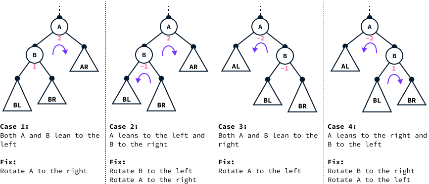
We implement these four cases in the .rebalance() method.
# Inside the AVLTree class

  def rebalance(self, node):
    if node is None:
      # Empty tree, no rebalancing needed
      return None
    balance = node.balance_factor()
    if abs(balance) <= 1:
      # The node is already balanced, no rebalancing needed
      return node
    if balance == 2:
      # Cases 1 and 2, the tree is leaning to the left
      if node.left.balance_factor() == -1:
        # Case 2, we first do a left rotation
        node.set_left(self.rotate_left(node.left))
      return self.rotate_right(node)
    # Balance must be -2
    # Cases 3 and 4, the tree is leaning to the left
    if node.right.balance_factor() == 1:
      # Case 4, we first do a right rotation
      node.set_right(self.rotate_right(node.right))
    return self.rotate_left(node)
Note that in each case, the method returns the root of the subtree that has just been balanced. This new subtree root will be used later to update the children during the rebalancing process.
Adding a node to an AVL tree is similar to the process in a regular BST, with the addition of restoring balance after the node is inserted. To add a node in a BST, we begin at the root and travel down the tree. At each step, we compare the value to be added with the current node's value. If the value to add is smaller, we move left; otherwise, we move right. While descending, we keep track of the parent node so we can insert the new node as its child.
Once we reach an empty node, there are two cases:
# Inside the AVLTree class
  def add(self, value):
    self.size += 1
    parent = None
    current = self.root
    while current is not None:
      parent = current
      if value < current.value:
        # Value to insert is smaller than node value, go left
        current = current.left
      else:
        # Value to insert is larger than node value, go right
        current = current.right
    # We found the parent, create the new node
    new_node = Node(value, parent)
    # Case 1: The parent is None so the new node is the root
    if parent is None:
      self.root = new_node
    else:
      # Case 2: Set the new node as a child of the parent
      if value < parent.value:
        parent.left = new_node
      else:
        parent.right = new_node
    # After a new node is added, we need to restore balance
    self.restore_balance(new_node)
The only difference between the .add() method of a BST and that of an AVL tree lies in the final step. This involves traversing back up the tree and rebalancing the nodes, starting from the newly added node to the root, and rebalancing each node by employing the .rebalance() method.
# Inside the AVLTree class
  def restore_balance(self, node):
    current = node
    # Go up the tree and rebalance left and right children
    while current is not None:
      current.set_left(self.rebalance(current.left))
      current.set_right(self.rebalance(current.right))
      current.update_heigth()
      current = current.parent
    self.root = self.rebalance(self.root)
    self.root.parent = None
Note that the .rebalance() method does nothing when the node is already balanced—it simply returns that same node. That’s why, while doing up the tree, we can call it on both sides, even though only one of them can be unbalanced. The other call simply leaves the tree unchanged.
Recall that we implemented the .rebalance() method so that it returns the (potentially) new root of the subtree. The reason for this was so that we could update the left and right children of the current nodes as we go up restoring balance.
The following diagram shows the steps of .restore_balance() going up the tree.
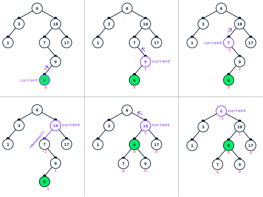
In the given example, we first add node 8. Then, the process of restoring balance begins at this node and works its way up the tree, checking and rebalancing the left and right children of each encountered node. This continues until node 10 is reached. Until this point, none of the invocations of the .rebalance() method have any effect, as the nodes remain balanced.
However, upon reaching node 10, it's observed that its left child, node 7, has a balance factor of -2, indicating a need for rebalancing. Consequently, .rebalance(7) is called, which results in the substitution of node 10's left child with the new root of the left subtree, node 8, effectively restoring balance to the tree.
Besides adding and deleting elements while maintaining the tree's balance, AVL trees support several other essential operations.
Due to the ordered nature of BST, the minimum value can be found at the leftmost node of the tree, whereas the maximum value is located at the rightmost node.
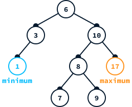
We have implemented two helper functions that identify the leftmost and rightmost nodes starting from a given node. These functions are useful for facilitating the implementation of node deletion.
# Inside the AVLTree class

  def leftmost(self, starting_node):
    # Find the leftmost node from a given starting node
    previous = None
    current = starting_node
    while current is not None:
      previous = current
      current = current.left
    return previous
  def minimum(self):
    # Return the minimum value in the tree
    if self.root is None:
      raise Exception("Empty tree")
    return self.leftmost(self.root).value
# Inside the AVLTree class
def rightmost(self, starting_node):
# Find the rightmost node from a given starting node
previous = None
current = starting_node
while current is not None:
previous = current
current = current.right
return previous
def maximum(self):
# Fidn the maximum value in the tree
if self.root is None:
raise Exception("Empty tree")
return self.rightmost(self.root).valueTo determine if a tree contains a specific value, we utilize the tree's order property to guide our search. Starting from the root, we traverse to the left if the value we seek is smaller than the current node and to the right if it's larger. If we reach the end of the tree without finding the desired value, it indicates that the value is not present in the tree.
To facilitate this process, we implement a helper method called .locate_node(). This method is particularly useful not only for searching but also for operations such as deleting values from the tree. Additionally, we use the .__contains__() method, which allows us to utilize the in operator to simplify checking for the presence of a value within the tree.
# Inside the AVLTree class

  def locate_node(self, value):

    # Returns the node containing a given value or None if no

    # such node exists

    current = self.root

    while current is not None:

      if value == current.value:

        return current

      if value < current.value:

        current = current.left

      else:

        current = current.right

    return None

  def __contains__(self, value):

    node = self.locate_node(value)

return node is not NoneDeleting a node in an AVL tree can be particularly challenging when the node is situated in the middle of the tree. If the node is a leaf, meaning it has no children, we can easily delete it by setting its parent's left or right child pointer to None based on whether the node is a left or right child.
A special case arises when the node targeted for deletion is the root of the tree. In this scenario, we can remove the node by setting the root to None.
# Inside the AVLTree class
def delete_leaf(self, node):
if node.parent is None:
self.root = None
elif node.is_left_child():
node.parent.left = None
node.parent = None
else:
node.parent.right = None
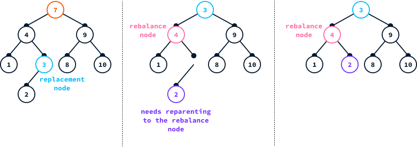
node.parent = NoneTo delete a value from an AVL tree, we must first locate the node containing that value using the .locate_node() method. Once the node is located, we can remove it with the .delete_leaf() method if it is a leaf node. If it's not a leaf node, direct removal would disrupt the tree's structure. To address this, we find a suitable replacement node. If the node to be deleted has a left child, we select the rightmost node in its left subtree. This approach ensures the tree maintains its ordered structure.
The diagram below exemplifies the removal of node 10 from a tree. Given it has a left child, we replace it with the rightmost node in the left subtree. Following the replacement, it's crucial to rebalance the tree, starting from the parent of the newly replaced node.
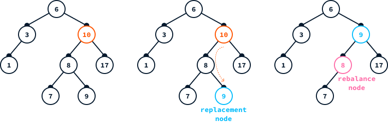
In this example, the replacement node is a leaf node. However, if the replacement node has children, it's necessary to reassign them to the parent of the replacement node. Since the replacement node is an extreme node (either the leftmost or the rightmost), it can have only one child. Therefore, this reassignment is always feasible.
# Inside the AVLTree class

  def delete(self, value):

    # Delete a value from the tree

    node = self.locate_node(value)

    if node is None:

      raise Exception("Value not stored in tree")

    replacement = None

    rebalance_node = node.parent

    if node.left is not None:

      # There's a left child so we replace with rightmost node

      replacement = self.rightmost(node.left)

      # Check if reparenting is needed

      if replacement.is_left_child():

        replacement.parent.set_left(replacement.left)

      else:

        replacement.parent.set_right(replacement.left)

    elif node.right is not None:

      # There's a right child so we replace with the leftmost node

      replacement = self.leftmost(node.right)

      # Check if reparenting is needed

      if replacement.is_left_child():

        replacement.parent.set_left(replacement.right)

      else:

        replacement.parent.set_right(replacement.right)

    if replacement:

      # We found a replacement so replace the value

      node.value = replacement.value

      rebalance_node = replacement.parent

    else:

      # No replacement so it means the node to delete is a leaf

      self.delete_leaf(node)

    if rebalance_node is not None:

      self.restore_balance(rebalance_node)
Range queries involve identifying all values that fall between two specified values. Due to the ordered nature of AVL trees, we can locate these values efficiently.
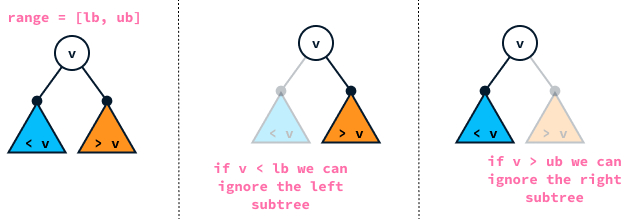
To locate all values within the range specified by lower bound lb and upper bound ub, we employ a recursive approach to search the tree. For each node encountered, if its value falls within this range, we include it in our results. Subsequently, we explore both the left and right subtrees to continue our search.
We ignore the left subtree if the node's value is less than the lower bound because all the values in the left subtree are smaller than the node's value. Similarly, we ignore the right subtree if the node's value is greater than the upper bound, as all values in the right subtree will be larger than the node's value.
  def search(self, node, lb, ub, results):

    # Search for values between lower bound and upper bound

    if node is None:

      return

    if lb <= node.value and node.value <= ub:

      results.append(node.value)

    if node.value >= lb:

      self.search(node.left, lb, ub, results)

    if node.value <= ub:

      self.search(node.right, lb, ub, results)

  def range_query(self, lb, ub):

    # Search for values between lower bound and upper bound

    results = []

    self.search(self.root, lb, ub, results)

return resultsWe have implemented an AVL tree capable of performing the following operations:
The avltree package package offers a Python implementation reflecting these capabilities.
Other self-balancing binary search trees, such as red-black trees, splay trees, and B-trees, provide similar functionalities. Generally, their performance is comparable across most applications, as they all maintain a guaranteed logarithmic height. However, AVL trees are more finely balanced, optimizing search operations at the cost of potentially slower insertions due to rigorous rebalancing requirements.
Splay trees are particularly effective in scenarios where recently accessed elements are frequently reused, making them an excellent choice for cache implementations.
B-trees are uniquely designed to operate efficiently on disk rather than in memory, making them invaluable for managing large data sets that exceed memory capacities, such as in database index creation.
There are several ways in which our implementation can be improved. Here are a few suggestions for exercises to deepen your understanding of AVL trees:
BSTs are a type of binary tree data structure that organizes data following a specific order. This organization allows for the avoidance of inspecting the entire dataset when searching for specific values. However, BSTs can become unbalanced, leading to deteriorated performance, which, in some scenarios, may necessitate inspecting the entire dataset.
AVL trees resolve this issue by enforcing additional balance properties through rotations. These properties ensure that the tree's height remains logarithmic in relation to the dataset's size, providing a significant improvement.
Logarithmic time complexity is a substantial enhancement over linear time complexity, making AVL trees incredibly efficient for query resolution. Even in datasets with billions of entries, AVL trees require the inspection of only a few data points to locate an element, making them considerably more efficient.
Learn data engineering with these courses!
Programa
Programa
Curso
Tutorial
Amberle McKee
Tutorial
Amberle McKee
Tutorial
François Aubry
Tutorial
Avinash Navlani
Tutorial
Zoumana Keita
Tutorial
Neetika Khandelwal