Makine Öğreniminde Düzenlileştirme: L1, L2 ve Elastic Net Açıklanıyor

Bir modeli öyle iyi eğittiniz ki eğitim örneklerinin neredeyse tamamında kusursuz, ama yeni veride başarısız mı? Hepimizin başına geldi.

Bu, aşırı uyumun (overfitting) yüksek seviyede bir tanımıdır. Model gerçek deseni öğrenmedi; bunun yerine eğitim verisini ezberledi. Üretimde, yeni ve görülmemiş verilerle, model güvenmeyeceğiniz tahminler yapar. Gerçek dünya verisi eğitim örneklerinden saptıkça bu sorun daha da büyür.

Düzenlileştirme bunu, kayıp fonksiyonuna bir ceza ekleyerek düzeltir. Bu ceza karmaşık modelleri caydırır. Başka bir deyişle, modelinizin her veri noktasına uymasını engelleyip genelleme yapmaya zorlayan mekanizmadır.

Bu yazıda, düzenlileştirmenin arkasındaki sezgiyi, en yaygın yöntemleri - L1, L2 ve Elastic Net - ve kullanım durumunuza göre doğru olanı nasıl seçeceğinizi anlatacağım.

Makine öğrenimi modellerinin üretimde neden ve nasıl başarısız olduğunu anlamak istiyorsanız, Önyargı-Varyans Dengesi blog yazımızı okuyun.

Makine Öğreniminde Düzenlileştirme (Regularization) Nedir

Düzenlileştirme, modelinizin karmaşıklığını caydırmak için kayıp fonksiyonuna bir ceza terimi ekleyen bir tekniktir.

Bu ceza terimi olmadan bir model, eğitim verisini istediği kadar yakından uyduracak esnekliğe sahiptir. Buna gürültü ve aykırı değerler de dahildir. Düzenlileştirme bu esnekliğe bir maliyet ekler. Model ne kadar karmaşık olmak isterse, o kadar yüksek ceza alır.

Modelinizin kayıp fonksiyonu normalde tahmin edilen ve gerçek değerler arasındaki farkı ölçer. Düzenlileştirme bu denkleme, modelin katsayıları büyüdükçe artan ekstra bir terim ekler. Model artık iki rakip hedefi dengelemek zorundadır: eğitim verisini uydurmak ve katsayıları küçük tutmak.

Bu denge, model esnekliğini kontrol eder.

Aşırı esnek bir model, eğitim verisini uydurmak için kendini her şekle sokabilir. Düzenlileştirme onu daha basit bir şekle geri düzeltir - bu da modelin daha önce görmediği verilerde de ayakta kalma olasılığını artırır.

Düzenlileştirme Neden Gerekli

Eğittiğiniz her model, iki kullanışsız modelin arasında bir yerde durur: biri fazla basit, diğeri fazla karmaşık.

Fazla basit bir model verinizdeki gerçek desenleri “anlamaz”. Sinyali kaçırır. Buna yetersiz uyum (underfitting) denir - model hem eğitim verisinde hem de yeni veride kötü performans gösterir.

Fazla karmaşık bir model ise tam tersini yapar. Eğitim verinizdeki her detayı, gürültü dahil, uydurur. Buna aşırı uyum (overfitting) denir - model eğitim verisinde harika performans gösterir, ancak yanlış şeyleri ezberlediği için yeni veride başarısız olur.

Somut bir örnek olarak polinom regresyonu ele alalım. Yumuşak bir eğri gösteren veriye 3. derece bir polinom uydurmak genellikle doğru desene uyduğunuz anlamına gelir. Ancak aynı veriye 15. derece bir polinom uydurmak aşırı uyuma yol açar - eğri her veri noktasından geçer ama aralarda rastgele tahminler yapar.

Aşağıdaki grafik bunun pratikte nasıl göründüğünü gösterir.

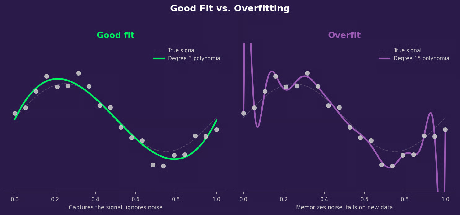
Tam kararında modele karşı fazla karmaşık model

Bu, önyargı-varyans dengesidir.

Basit modeller yüksek önyargıya sahiptir - gerçek desenleri kaçıran güçlü varsayımlar yaparlar. Karmaşık modeller ise yüksek varyansa sahiptir - gördükleri belirli eğitim örneklerine aşırı duyarlıdırlar ve verideki küçük değişiklikler çok farklı modellere yol açar.

Düzenlileştirme, ikisinin de en iyisini elde etmenize yardımcı olur. Karmaşıklığı ortadan kaldırmaz, ancak cezalandırır. Sonuç olarak, modelinizin gerçek sinyali öğrenme şansı artar.

Düzenlileştirme Nasıl Çalışır

Her model, kayıp fonksiyonunu - tahminlerinin ne kadar hatalı olduğunu ölçen bir metriği - en aza indirerek öğrenir. Düzenlileştirme olmadan modelin tek işi bu hatayı en aza indirmektir. Bunu yapmak için, eğitim verisini uyduran ancak genelleştiremeyen büyük katsayılar da dahil olmak üzere ne gerekiyorsa yapar.

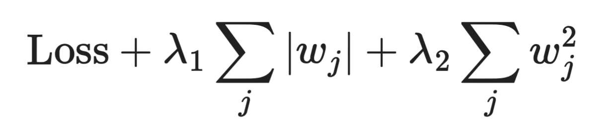
Düzenlileştirme amacı değiştirir. Artık yalnızca hatayı en aza indirmek yerine, model şunu en aza indirir:

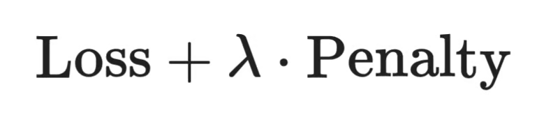
Düzenlileştirme nasıl çalışır

Ceza terimi, modelin katsayılarının bir fonksiyonudur. Büyük katsayılar cezayı artırır. Toplam maliyeti düşük tutmak için model katsayılarını küçük tutmaya zorlanır - bu da daha basit, daha iyi genelleştirilebilir çözümler anlamına gelir.

λ (lambda), cezanın ne kadar önemli olduğunu kontrol eder. Daha yüksek λ, model üzerinde basit kalması yönünde daha fazla baskı oluşturur. Daha düşük λ, modelin veriyi uydurmaya daha çok odaklanmasına izin verir. Bunu, aşağıdaki Düzenlileştirme Gücünü Seçme bölümünde nasıl ayarlayacağınızı göreceksiniz.

Makine Öğreniminde Düzenlileştirme Türleri

Model karmaşıklığını cezalandırmanın birkaç yolu vardır. Her biri katsayılara farklı şekilde baskı uygular; bu da farklı durumlara uygun oldukları anlamına gelir.

L2 düzenlileştirme (Ridge regresyon)

L2 düzenlileştirme, her bir katsayının karesini cezalandırır. Bir katsayı ne kadar büyükse, cezaya o kadar fazla katkıda bulunur - ve model onu küçültmek için o kadar çok çabalar.

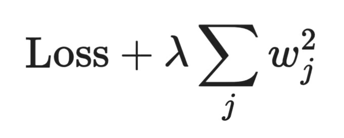
L2 düzenlileştirme

Buradaki kilit kelime küçültmektir. L2, tüm katsayıları sıfıra doğru iter, ancak asla tam olarak sıfıra ulaşmaz. Her özellik modelde kalır, yalnızca daha küçük bir ağırlıkla. Bu, Ridge'i, çoğu özelliğinizin ilgili olduğuna inandığınız ve dengeli, kararlı bir model istediğiniz durumlar için iyi bir varsayılan yapar.

L1 düzenlileştirme (Lasso regresyon)

L1 düzenlileştirme, kare yerine her bir katsayının mutlak değerini cezalandırır.

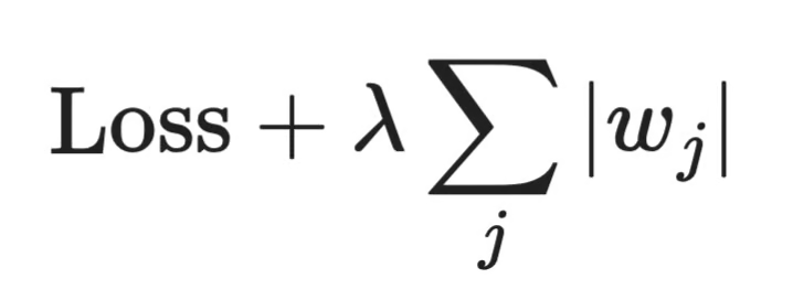
L1 düzenlileştirme

Bu küçük fark büyük bir sonuca yol açar. L1, katsayıları tam olarak sıfıra kadar itebilir; bu da özellikleri modelden kaldırdığı anlamına gelir. Bunu otomatik özellik seçimi gibi düşünebilirsiniz. Başka bir deyişle, Lasso düzenlileştirme, özellikleri kaldırarak modelinizi basitleştirebilir.

L1 ve L2 düzenlileştirme karşılaştırması

Temel fark, seyrekliğe dayanır. L1, seyrek modeller üretir - yalnızca bir alt küme özellik geçer. L2, yoğun modeller üretir - tüm özellikler kalır, ancak daha küçük ağırlıklarla.

Bu, yorumlanabilirliği de etkiler. 5 etkin özellikle bir Lasso modeli, katkı sağlayan 50 özelliğin bulunduğu bir Ridge modelinden daha kolay açıklanır. Ancak Ridge, özellikler birbiriyle korelasyonlu olduğunda daha kararlı olma eğilimindedir; çünkü ağırlığı, rastgele birini seçmek yerine aralarında dağıtır.

İşte farkların hızlı bir özeti:

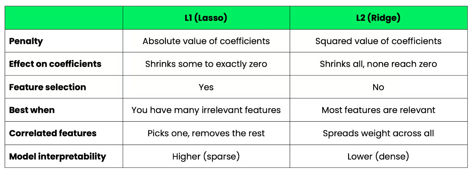
L1 ve L2 düzenlileştirme

Bunların Python'da nasıl karşılaştırıldığına bakmak isterseniz, Python'da Lasso ve Ridge Regresyonu eğitimimiz size yardımcı olur.

Elastic Net düzenlileştirme

Elastic Net, L1 ve L2'yi tek bir ceza teriminde birleştirir.

Elastic Net düzenlileştirme

Amaç, her ikisinin de en iyisini elde etmektir: L1'in özellik seçimi ve L2'nin kararlılığı. Bu, korelasyonlu özelliklere sahip olduğunuzda ve hâlâ bazılarını elemek istediğinizde kullanışlıdır. Lasso tek başına, korelasyonlu bir gruptan genellikle bir özelliği seçer ve geri kalanını görmezden gelir. Elastic Net ise ilgisiz olanları kaldırırken birkaçını tutma olasılığı daha yüksektir.

Farklı Modellerde Düzenlileştirme

Düzenlileştirme birçok makine öğrenimi modelinde karşımıza çıkar, ancak farklı biçimlerde. Bunların neler olduğuna bakalım.

Doğrusal regresyon, çoğu kişinin düzenlileştirmeyi ilk gördüğü yerdir. Doğrusal regresyona L2 düzenlileştirme eklediğinizde Ridge düzenlileştirme elde edersiniz. Benzer şekilde, L1 eklemek Lasso regresyonu verir. Matematik, yukarıda anlatıldığıyla aynıdır - en küçük kareler kaybına bir ceza terimi eklenir.

Lojistik regresyon aynı şekilde çalışır. Kayıp fonksiyonu değişir - kare hata yerine çapraz entropidir - ancak ceza terimi aynıdır. Çoğu makine öğrenimi kütüphanesi, varsayılan olarak lojistik regresyona L2 düzenlileştirme uygular; bu nedenle scikit-learn'de C adlı bir parametre görürsünüz. Bu, λ'nın tersidir; dolayısıyla daha küçük bir C, daha güçlü düzenlileştirme anlamına gelir.

Sinir ağları birkaç farklı yaklaşım kullanır:

• Ağırlık çürümesi (weight decay): Ağın ağırlıklarına uygulanan L2 düzenlileştirme - aynı şekilde çalışır, sadece çok daha büyük ölçekte
• Dropout: Eğitim sırasında, her geçişte nöronların bir kısmını rastgele devre dışı bırakır; bu da ağın katmanlar boyunca tek bir yola aşırı bağımlı olmasını engeller.

Her ikisi de aşırı uyumu azaltır, ancak farklı yollarla.

Ağaç tabanlı modeller ise hiç kayıp cezası kullanmaz. Bunun yerine karmaşıklığı budamayla kontrol ederler - bir ağacın ne kadar derin büyüyebileceğini sınırlamak veya tahminleri yeterince iyileştirmeyen dalları kaldırmak gibi. scikit-learn'deki max_depth ve min_samples_split gibi hiperparametreler, adı böyle olmasa da düzenlileştirme parametreleridir.

Düzenlileştirme ve Önyargı-Varyans Dengesi

Düzenlileştirme tamamen uzlaşmalarla ilgilidir.

Bir ceza terimi eklediğinizde, modelin yapabileceklerini kısıtlarsınız. Artık eğitim verisini istediği kadar yakından uyduramaz. Bu kısıt, önyargı doğurur - model tasarım gereği biraz yanlış varsayımlar yapar, çünkü ona basit kalmasını söylediniz.

Ancak aynı kısıt, varyansı azaltır. Her veri noktasını uyduramayan bir model, üzerinde eğitildiği belirli örneklere daha az duyarlıdır. Biraz farklı bir veri kümesi üzerinde eğittiğinizde benzer bir sonuç alırsınız. Üretimde modelinizin başarısız olmaması için asıl istediğiniz bu kararlılıktır.

Düzenlileştirme olmadan, düşük önyargıya (az varsayım yapar ve eğitim verisini iyi uydurur) ve yüksek varyansa (eğitim verisindeki küçük değişiklikler çok farklı modellere yol açar; bu da yeni veride güvenilemeyeceği anlamına gelir) sahip, son derece esnek bir model elde edersiniz.

Düzenlileştirme dengeyi kaydırmakla ilgilidir. Daha az varyans karşılığında biraz daha fazla önyargı, genellikle modelin görmediği veride daha iyi performansa yol açar. Uzlaşma budur ve neredeyse her zaman yapmaya değerdir.

Düzenlileştirme Gücünü Seçme

Bir makine öğrenimi uygulayıcısı olarak, düzenlileştirme türünü seçtikten sonra düzenlileştirme gücünü ayarlamanız gerekir.

Bu güç, genellikle matematiksel gösterimde lambda (λ) veya scikit-learn'de alpha olarak adlandırılan bir hiperparametre ile kontrol edilir. Ceza teriminin önündeki çarpandır. Bunu değiştirdiğinizde, modelin sadeliğe ne kadar zorlandığını değiştirirsiniz.

Bunu her iki yönde de yanlış ayarlarsanız, üretimde sorun yaşarsınız:

• Çok düşük: ceza, etkili olacak kadar güçlü değildir. Model, hiç düzenlileştirme yokmuş gibi aşırı uyum yapar.
• Çok yüksek: ceza baskın faktördür. Model öylesine kısıtlanır ki, verideki gerçek desenleri anlayamaz. Bu da yetersiz uyumdur.

Doğru değer ikisinin arasında bir yerde bulunur ve evrensel bir cevap yoktur. Verinize, modelinize ve uğraştığınız gürültü miktarına bağlıdır.

Bunu bulmanın standart yolu çapraz doğrulamadır. Eğitim verinizi katlara bölersiniz, her kat kombinasyonunda modeli eğitirsiniz ve bir dizi alpha değeri üzerinde doğrulama performansını ölçersiniz. En iyi ortalama doğrulama puanını veren değeri kullanırsınız.

scikit-learn'de RidgeCV ve LassoCV bunu otomatik olarak yapabilir - alpha değerleri üzerinde çapraz doğrulama çalıştırır ve sizin için en iyisini seçer.

from sklearn.linear_model import RidgeCV

model = RidgeCV(alphas=[0.01, 0.1, 1.0, 10.0], cv=5)
model.fit(X_train, y_train)

print(model.alpha_)

Yazdırılan alpha, çapraz doğrulama ile bulunan en iyi değeri gösterecektir. Geniş bir değer aralığıyla başlayın, ardından en iyi aralığın nerede olduğunu öğrendikten sonra daraltın.

Sonuç

Düzenlileştirme, bir modelin kendi iyiliği için fazla “zeki” olmasını engellemenin yoludur.

Karmaşıklığı cezalandırır ve bu da modeli, eğitim verisini ezberlemek yerine genelleyen çözümler bulmaya zorlar. L2, tüm özelliklerinizi korur ve etkilerini azaltır. L1, ilgisiz özellikleri kaldırır. Elastic Net ikisini birleştirir. Ve doğrusal modeller, lojistik regresyon, sinir ağları ve ansambıl (ensemble) modeller arasında aynı fikir farklı biçimlerde karşımıza çıkar ve her zaman “düzenlileştirme” olarak adlandırılmaz.

En önemlisi, seçtiğiniz teknik ve ayarladığınız güçtür. Bu yüzden yapmanız gereken şey denemektir. Farklı parametre değerleriyle farklı yaklaşımları deneyin. Birini seçip geçmeyin.

Veriniz neyin işe yaradığını söyleyecektir.

Daha fazla düzenlileştirme tekniğini uygulamalı olarak görmek istiyorsanız, Python ile Makine Öğrenimi Bilimcisi eğitim yolumuza kaydolun. Sizi işe hazır hale getirecek 85 saatlik materyal içerir.