Comment actualiser un tableau croisé dynamique : Excel et Google Sheets

Vous avez enfin terminé la création de votre rapport idéal, et un tableau croisé dynamique clair présente les ventes par région, par produit et par mois. Tout semble donc parfait.

Ensuite, votre collègue met à jour la source de données. Vous ouvrez à nouveau le fichier et vous vous attendez à ce que les nouveaux chiffres apparaissent, mais rien ne change.

Vos totaux sont incorrects. Les nouvelles entrées ne sont pas disponibles. Et maintenant, vous vous demandez si vous avez commis une erreur.

Voici ce que vous devez savoir : Excel et Google Sheets utilisent un cache Pivot, qui est essentiellement un instantané enregistré de vos données. Cela permet à votre tableau croisé dynamique de se charger plus rapidement, mais il ne se met pas automatiquement à jour lorsque les données changent.

Dans ce guide, je vais vous expliquer comment actualiser manuellement vos tableaux croisés dynamiques, que vous travailliez dans Excel ou Google Sheets.

Comment actualiser un tableau croisé dynamique

Explorons quelques méthodes pour actualiser le tableau croisé dynamique dans Excel et Google Sheets.

Actualisation d'un tableau croisé dynamique dans Excel

Il existe trois méthodes pour actualiser un tableau croisé dynamique dans Excel : 

Méthode manuelle

Voici comment procéder manuellement : 

1. Veuillez cliquer n'importe où dans votre tableau croisé dynamique.
2. Veuillez consulter les onglet Données dans le ruban supérieur.
3. Veuillez cliquer sur Actualiser tout (ou simplement Actualiser, selon votre version d'Excel).

Une fois cette opération effectuée, Excel met à jour votre tableau croisé dynamique à l'aide des dernières données de votre feuille source.

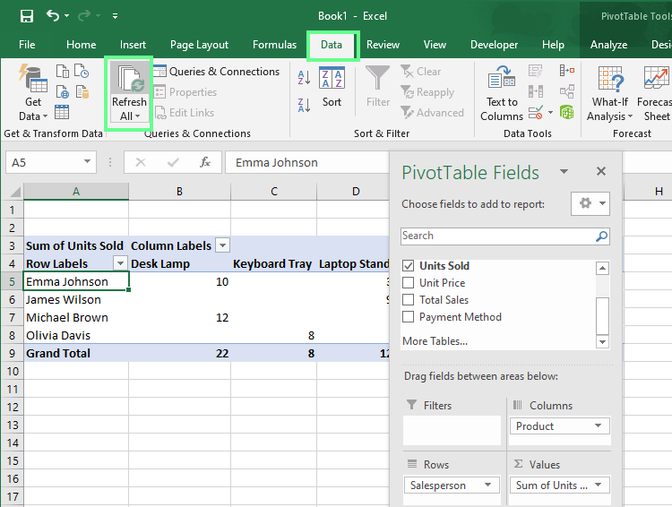
Veuillez actualiser manuellement le tableau croisé dynamique. Image fournie par l'auteur.

s utiles: Si votre classeur contient plusieurs tableaux croisés dynamiques provenant de différents ensembles de données, veuillez utiliser la fonction «Actualiser tout » d' .

Raccourcis clavier

Si vous appréciez autant que moi l'utilisation des touches, il existe une méthode plus rapide : Veuillez appuyer sur « Alt + F5 » pour actualiser le tableau croisé dynamique sélectionné.

Si vous souhaitez actualiser tous les tableaux croisés dynamiques de votre classeur, veuillez appuyer sur la combinaison de touches Ctrl+ Ctrl + Alt + F5.

Actualisation automatique

Vous pouvez également configurer Excel pour qu'il actualise votre tableau croisé dynamique à chaque ouverture du fichier :

1. Veuillez cliquer n'importe où dans votre tableau croisé dynamique.
2. Veuillez vous rendre sur Analyser > Tableau croisé dynamique > Options. (Ou cliquez avec le bouton droit sur votre tableau croisé dynamique et sélectionnez Options du tableau croisé dynamique)
3. Dans les boîte de dialogue Options du tableau croisé dynamique , veuillez vous rendre dans l'onglet onglet Données .
4. Veuillez cocher la case pour Actualiser les données à l'ouverture du fichier.
5. Veuillez cliquer ici OK.

Désormais, chaque fois que vous ouvrirez votre classeur, Excel récupérera les données les plus récentes pour vous.

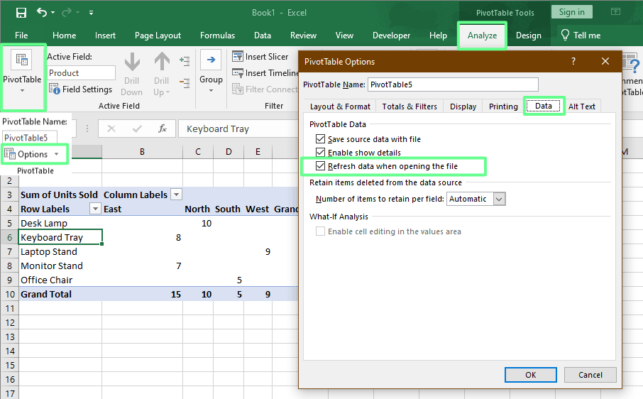
Veuillez configurer l'actualisation automatique du tableau croisé dynamique. Image fournie par l'auteur.

Actualisation d'un tableau croisé dynamique dans Google Sheets

Dans Google Sheets, les tableaux croisés dynamiques (Google écrit cette expression avec un espace) se mettent à jour automatiquement lorsque vos données sources changent.

Par exemple, si vous apportez des modifications à vos données, puis que vous consultez votre tableau croisé dynamique, vous constaterez que celui-ci reflète automatiquement ces modifications. Il n'est pas nécessaire de cliquer sur« Actualiser » ( ) ou d'effectuer une action particulière.

Options d'automatisation

Si vous mettez régulièrement à jour les données, l'actualisation manuelle peut devenir difficile. Heureusement, Excel et Google Sheets vous permettent d'automatiser le processus, afin que vos tableaux croisés dynamiques (ou tableaux pivot) restent à jour sans nécessiter de clics supplémentaires.

Dans Excel

Il existe trois méthodes pour automatiser le processus de rafraîchissement dans Excel.

Automatisation VBA

Si vous maîtrisez les macros, vous pouvez utiliser VBA (Visual Basic for Applications) pour actualiser automatiquement les tableaux croisés dynamiques :

1. Veuillez appuyer sur Alt + F11 pour ouvrir l'éditeur VBA.

2. Veuillez cliquer ici Insérer > Module.

3. Veuillez copier ce code simple :

Sub AutoRefreshPivotTables()
    Dim PT As PivotTable
    Dim WS As Worksheet
    For Each WS In ThisWorkbook.Worksheets
        For Each PT In WS.PivotTables
            PT.PivotCache.Refresh
        Next PT
    Next WS
End Sub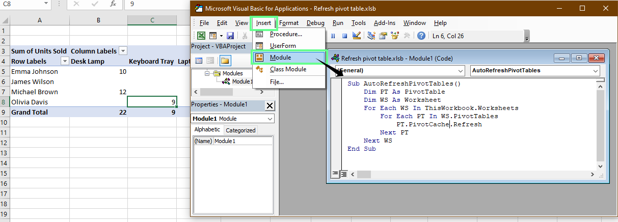

4. Veuillez fermer l'éditeur.
5. Désormais, lorsque vous ouvrirez le classeur, le tableau croisé dynamique sera automatiquement actualisé. 

Veuillez actualiser le tableau croisé dynamique à l'aide de VBA. Image fournie par l'auteur.

Actualisation de la requête de données

Si votre tableau croisé dynamique est connecté à Power Query, vous pouvez actualiser à la fois vos données et vos tableaux croisés dynamiques en une seule étape : 

Veuillez vous rendre sur Données > Actualiser tout.

Cela met à jour votre requête et tous les tableaux croisés dynamiques connectés.

Conseil de professionnel : Sous Données > Requêtes et connexions, sur le côté droit, vous trouverez le panneaud'sRequêtes et connexions . Veuillez cliquer avec le bouton droit de la souris et sélectionner «Propriétés d' » ( ). Veuillez cli Ici, vous pouvez programmer des actualisations.

Utilisation de Power Query pour mettre à jour les tableaux croisés dynamiques. Image fournie par l'auteur.

Connexions de données externes

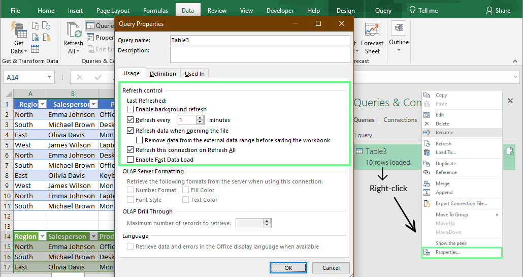
Si votre tableau croisé dynamique extrait des données provenant de sources externes (telles qu'une base de données, un fichier CSV ou un flux Web), Excel peut le mettre à jour automatiquement. Voici comment procéder pour configurer cela :

• Veuillez vous rendre sur Données > Connexions > Propriétés.

• Dans le onglet Utilisation , veuillez cocher la case Actualiser les données lors de l'ouverture du fichier.

• Veuillez vérifier l'actualisation de toutes les n minutes si vous souhaitez qu'elle se mette à jour automatiquement. (Facultatif) 

Cette configuration convient aux tableaux de bord qui s'appuient sur des données en temps réel ou des importations quotidiennes.

Dans Google Sheets

Dans Google Sheets, il n'est pas nécessaire d'automatiser quoi que ce soit à l'aide de Apps Script ou des modules complémentaires, car le tableau croisé dynamique est mis à jour automatiquement.

Si vous ajoutez de nouvelles colonnes ou lignes, veuillez simplement étendre la plage de données ou les insérer entre les colonnes ou lignes existantes, et Google Sheets mettra tout à jour automatiquement.

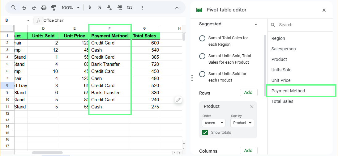
Éditeur de tableau croisé dynamique dans Google Sheets. Image fournie par l'auteur.

Dépannage des actualisations de tableaux croisés dynamiques

Même lorsque tout est correctement configuré, il arrive parfois que votre tableau croisé dynamique ne s'actualise pas comme prévu. Examinons quelques raisons courantes pour lesquelles cela se produit et comment vous pouvez résoudre ces problèmes dans Excel et Google Sheets.

Dans Excel

Voici comment résoudre les problèmes liés aux tableaux croisés dynamiques dans Excel :

Vérifier les références de plage et le cache pivot

Si votre tableau croisé dynamique n'affiche pas les nouvelles données, il est possible que votre plage de données n'inclue pas les dernières lignes. Pour résoudre ce problème :

• Veuillez cliquer n'importe où dans le tableau croisé dynamique «». Veuillez vous rendre sur Analyser > Modifier la source de données et assurez-vous que la plage couvre l'ensemble de vos données.

• Veuillez convertir votre plage de données en tableau (Ctrl + T) car les tableaux étendent automatiquement le tableau croisé dynamique lorsque vous ajoutez de nouvelles lignes après l'actualisation.

• Si votre tableau croisé dynamique ne se met toujours pas à jour, il est possible que le cache pivot soit obsolète. Veuillez essayerDonnées > Actualiser tout dans l' .

Reconnecter les sources de données externes

Il arrive parfois que votre tableau croisé dynamique ne puisse pas être actualisé car la source de données à laquelle il est lié, telle qu'une base de données, un fichier Power Query ou une feuille en ligne, est hors ligne ou a été déplacée :

• Veuillez vous rendre sur Données > Connexions.
• Veuillez vérifier l'état de chaque connexion répertoriée.
• Si l'un d'entre eux apparaît comme inactif ou manquant, veuillez cliquer pour vous reconnecter ou mettre à jour le chemin d'accès au fichier.
• Une fois la connexion rétablie, veuillez cliquer sur Actualiser tout pour recharger les dernières données.

s utiles: Si le fichier de données a été renommé ou déplacé, veuillez mettre à jour le lien directement dans les propriétés de connexion afin qu'il ne soit pas à nouveau rompu.

Réduire le délai de rafraîchissement pour les ensembles de données volumineux

Si votre classeur met trop de temps à s'actualiser, veuillez suivre les étapes suivantes :

• Veuillez désactiver temporairement les calculs automatiques (Formules > Options de calcul > Manuel), puis actualisez.
• Divisez les tableaux croisés dynamiques de grande taille en tableaux plus petits, filtrés par région, produit ou mois.
• Veuillez supprimer les champs ou les totaux inutiles qui ralentissent le traitement.

Dans Google Sheets

Bien que les tableaux croisés dynamiques dans Google Sheets s'actualisent généralement automatiquement, il arrive parfois qu'ils n'affichent pas les derniers chiffres. Examinons deux causes courantes et comment les résoudre.

Veuillez vérifier la référence de la gamme.

Si vous ajoutez de nouvelles lignes ou colonnes en dehors de la plage de données d'origine sur laquelle votre tableau croisé dynamique a été créé, Sheets ne les inclura pas automatiquement.

Par exemple, vous avez ajouté une nouvelle colonne intitulée Mode de paiement à droite de l'ensemble de données, mais le tableau croisé dynamique ne l'a pas détectée :

• Veuillez ouvrir l'éditeur de tableau croisé dynamique et ajuster la plage. 
• Lors de la création de votre tableau croisé dynamique, veuillez sélectionner une plage légèrement plus grande que vos données actuelles.
• Si vous devez ajouter de nouvelles lignes ou colonnes ultérieurement, veuillez les insérer dans la plage existante plutôt qu'au-delà.

Par exemple, si votre plage actuelle est A1:C11, veuillez ne pas ajouter une nouvelle colonne dans D.. Veuillez plutôt insérer une nouvelle colonne entre A et C, afin que la nouvelle colonne reste dans la plage.

De cette manière, votre tableau croisé dynamique sera toujours mis à jour automatiquement.

Supprimer les filtres 

Il peut arriver que votre tableau croisé dynamique n'affiche pas les derniers chiffres, même si vos données ont été modifiées. Ceci se produit généralement lorsqu'un filtre est activé.

Par exemple, vous avez peut-être défini un filtre pour n'afficher que les articles dont les ventes sont supérieures à 50. Ensuite, vous mettez à jour les ventes d'un article de 25 à 130, mais il n'apparaît toujours pas dans le rapport. En effet, le filtre empêche la visibilité :

• Veuillez vous rendre sur Données > cliquez sur Supprimer le filtre pour le désactiver.
• Veuillez vérifier votre tableau croisé dynamique pour confirmer que la mise à jour apparaît désormais.
• Une fois que tout semble correct, veuillez réappliquer votre filtre si nécessaire.

Lorsque vous désactivez puis réactivez le filtre, Google Sheets est contraint de revérifier vos données et d'afficher les valeurs les plus récentes.

Conclusions finales 

Une petite mise à jour peut faire toute la différence. Il garantit l'exactitude de vos rapports et veille à ce que les chiffres affichés reflètent vos données les plus récentes.

Vous pouvez mettre à jour vos tableaux manuellement, utiliser un raccourci ou configurer une automatisation si vous souhaitez gagner du temps. N'oubliez pas de vous inscrire à nos cours spécialisés si vous souhaitez approfondir vos compétences. Je recommande vivement les cours « Analyse de données dans Excel » et « Introduction à Power Query dans Excel ».