
Course
Data Preparation in Excel
3 hr
85.3K
You finally finish building your perfect report, and a neat PivotTable shows sales by region, product, and month. So everything looks great.
Then your teammate updates the data source. You open the file again and expect that the new numbers will appear, but nothing changes.
Your totals are off. The new entries are missing. And now you’re wondering if you did something wrong.
Here’s what you need to know: Excel and Google Sheets use a Pivot cache, which is basically a stored snapshot of your data. It helps your PivotTable load faster, but it doesn’t automatically update when the data changes.
In this guide, I’ll walk you through how to refresh your PivotTables manually, whether you are working in Excel or Google Sheets.
Let’s explore a few ways to refresh the PivotTable in Excel and Google Sheets.
There are three ways to refresh a PivotTable in Excel:
Here’s how you can do it manually:
Once done, Excel updates your PivotTable using the latest data from your source sheet.
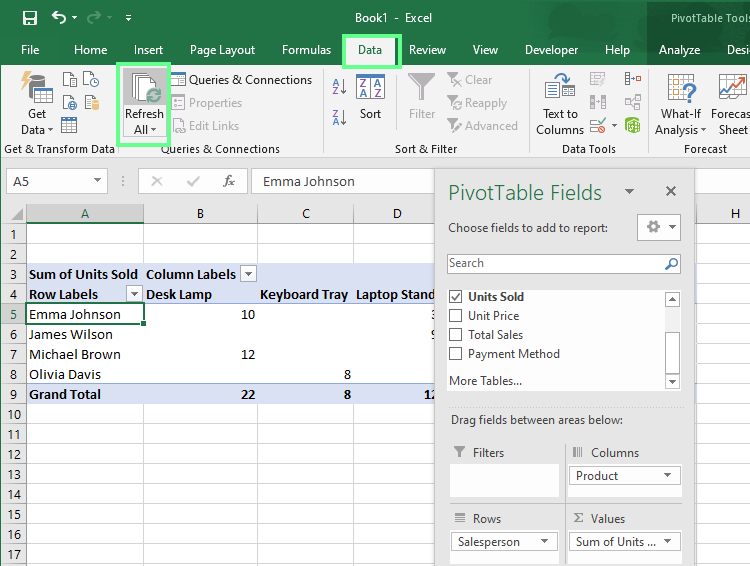
Manually refresh the PivotTable. Image by Author.
Tip: If you have more than one PivotTable of different datasets in your workbook, Refresh All updates.
If you like using keys as much as I do, there’s a faster way: Press Alt + F5 to refresh the selected PivotTable.
If you need to refresh all PivotTables in your workbook, press Ctrl + Alt + F5 instead.
You can also make Excel refresh your PivotTable each time you open a file:
Now, each time you open your workbook, Excel will pull the latest data for you.
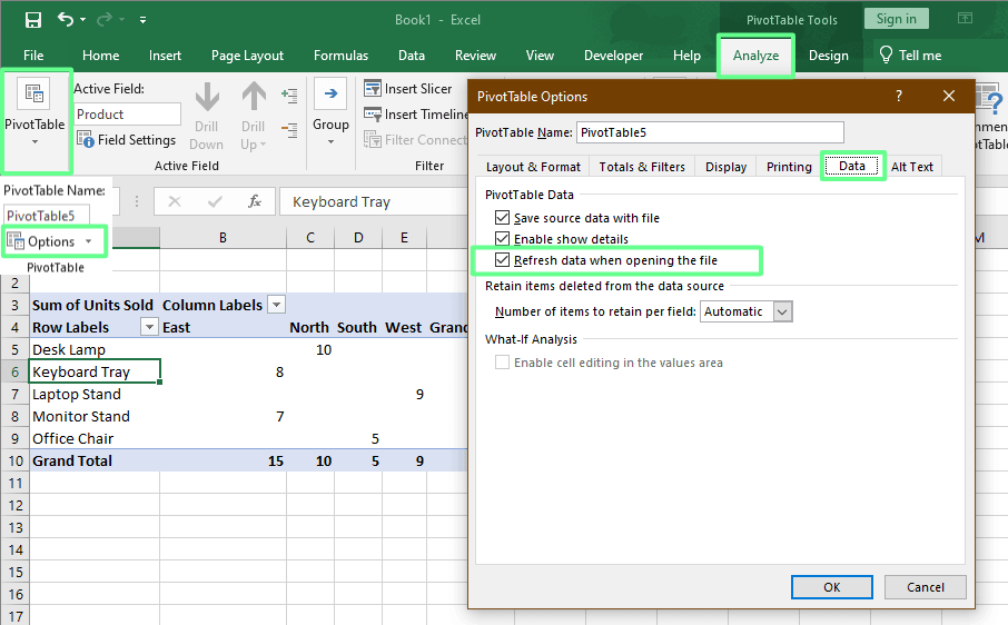
Set the auto refresh of the pivot table. Image by Author.
In Google Sheets, Pivot tables (Google writes this with a space) update automatically when your source data changes.
For example, if you make some changes in your data and then look at your PivotTable, you will see that the PivotTable automatically reflects the changes. You don’t have to click Refresh or do anything special.
If you regularly update data, manual refreshing may become hard. Luckily, both Excel and Google Sheets allow you to automate the process, so your PivotTables (or Pivot Tables) stay up to date without requiring extra clicks.
There are three ways to automate the refresh process in Excel.
If you’re comfortable with macros, you can use VBA (Visual Basic for Applications) to refresh PivotTables automatically:
Press Alt + F11 to open the VBA editor.
Click Insert > Module.
Paste this simple code:
Sub AutoRefreshPivotTables()
    Dim PT As PivotTable
    Dim WS As Worksheet
    For Each WS In ThisWorkbook.Worksheets
        For Each PT In WS.PivotTables
            PT.PivotCache.Refresh
        Next PT
    Next WS
End Sub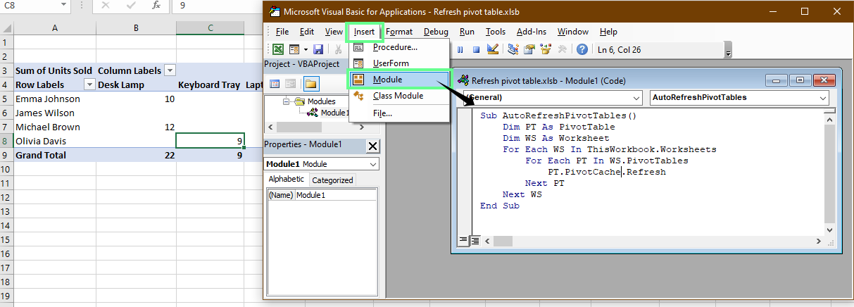
Refresh the PivotTable using VBA. Image by Author.
If your PivotTable is connected to Power Query, you can refresh both your data and PivotTables in one step:
Go to Data > Refresh All.
This updates your query and every connected PivotTable.
Pro tip: Under Data > Queries & Connections, on the right side, you’ll see the Queries & Connections panel. Right-click and select Properties. Here, you can schedule refreshes.
Using Power Query to update PivotTables. Image by Author.
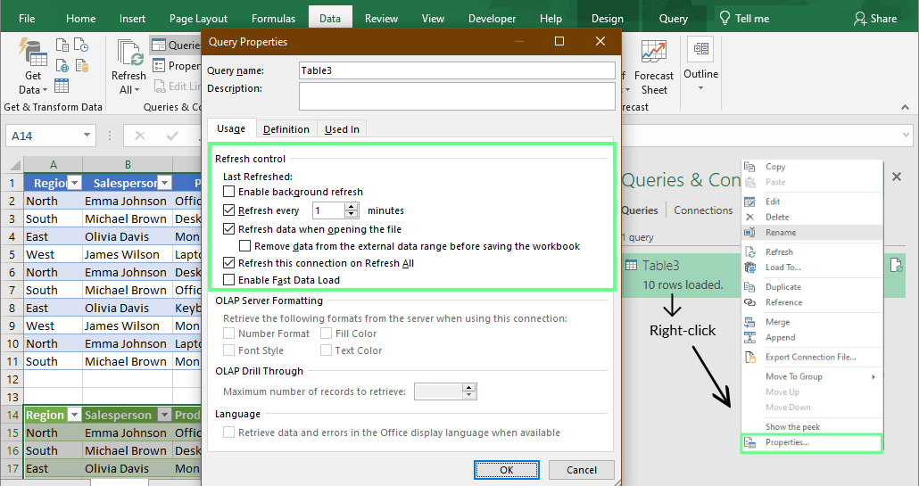
If your PivotTable pulls data from external sources (like a database, CSV, or web feed), Excel can update it automatically. Here’s how you can set this up:
Go to Data > Connections > Properties.
In the Usage tab, check Refresh data when opening the file.
Check Refresh every n minutes if you want it to update on a timer. (Optional)
This setup is suitable for dashboards that rely on live data or daily imports.
In Google Sheets, you don’t have to automate anything using Apps Script or add-ons because it automatically updates the PivotTable.
If you add new columns or rows, just expand the data range or insert them between existing columns or rows, and Google Sheets will update everything on its own.
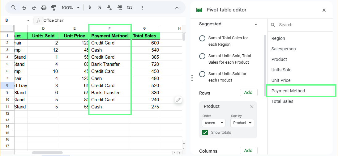
Pivot table editor in Google Sheets. Image by Author.
Even with everything set up correctly, sometimes your PivotTable doesn’t refresh the way you expect. Let's see some common reasons why this happens and how you can fix these issues in both Excel and Google Sheets.
Here’s how you can troubleshoot PivotTable-related issues in Excel:
If your PivotTable isn’t showing new data, your data range might not include the latest rows. To fix this:
Ctrl + T) because tables automatically expand the PivotTable as you add new rows after refreshing.Sometimes your PivotTable can’t refresh because the data source it’s linked to, such as a database, Power Query file, or online sheet, has gone offline or moved:
Tip: If the data file was renamed or relocated, update the link directly in the connection properties so it doesn’t break again.
If your workbook takes too long to refresh, do the following:
Even though Pivot Tables in Google Sheets usually refresh automatically, sometimes they still don’t show the latest numbers. Let’s look at two common reasons and how to fix them.
If you add new rows or columns outside the original data range your PivotTable was built on, Sheets won’t include them automatically.
For example, you added a new column called Payment Method to the right of the dataset, but the PivotTable didn’t see it:
For example, if your current range is A1:C11, don’t add a new column in D. Instead, insert a new column between A and C, so the new column stays inside the range.
This way, your PivotTable will always update automatically.
Sometimes your Pivot Table may not show the latest numbers even though your data has changed. This usually happens when a filter is active.
For example, you may have set a filter to only show items with sales greater than 50. Then you update an item’s sales from 25 to 130, but it still doesn’t appear in the report. That’s because the filter is blocking the view:
When you turn the filter off and on again, it forces Google Sheets to recheck your data and display the most recent values.
A quick refresh can make all the difference. It keeps your reports accurate and ensures the numbers you see reflect your latest data.
You can update your tables manually, use a shortcut, or set up automation if you want to save time. Remember to enroll in our dedicated courses if you want to take your skills a step further. I recommend Data Analysis in Excel and our Introduction to Power Query in Excel courses.
Learn with DataCamp
Course
Course
Course
Tutorial
Aditya Sharma
Tutorial
Laiba Siddiqui
Tutorial
Elena Kosourova
Tutorial
Javier Canales Luna
Tutorial
Rajesh Kumar
Tutorial
Javier Canales Luna