By now, you'll already know the Pandas library is one of the most preferred tools for data manipulation and analysis, and you'll have explored the fast, flexible, and expressive Pandas data structures, maybe with the help of DataCamp's Pandas Basics cheat sheet.
Yet, there is still much functionality that is built into this package to explore, especially when you get hands-on with the data: you'll need to reshape or rearrange your data, iterate over DataFrames, visualize your data, and much more. And this might be even more difficult than "just" mastering the basics.
That's why today's post introduces a new, more advanced Pandas cheat sheet.
It's a quick guide through the functionalities that Pandas can offer you when you get into more advanced data wrangling with Python.
(Do you want to learn more? Start our Data Manipulation with pandas course for free now or try out our Pandas DataFrame tutorial! )
Have this cheat sheet at your fingertips
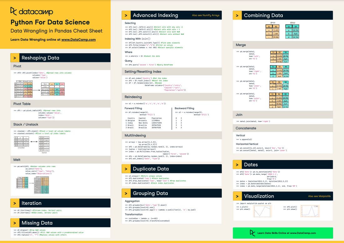
Download PDFThe Pandas cheat sheet will guide you through some more advanced indexing techniques, DataFrame iteration, handling missing values or duplicate data, grouping and combining data, data functionality, and data visualization.
In short, everything that you need to complete your data manipulation with Python!
Don't miss out on our other cheat sheets for data science that cover Matplotlib, SciPy, Numpy, and the Python basics.
Reshape Data
Pivot
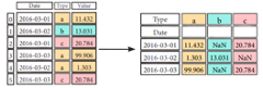
>>> df3= df2.pivot(index='Date', #Spread rows into columns columns='Type', values='Value')Stack/ Unstack

>>>stacked= df5.stack() #Pivot a level of column labels>>> stacked.unstack() #Pivot a level of index labelsMelt
>>> pd.melt(df2, #Gather columns into rows id_vars=[''Date''], value_vars=[''Type'', ''Value''], value name=''Observations'')Iteration
>>> df.iteritems() #{Column-index, Series) pairs>>> df.iterrows() #{Row-index, Series) pairsMissing Data
>>> df.dropna() #Drop NaN values>>> df3.fillna(df3.mean()) #Fill NaN values with a predetermined value>>> df2.replace("a", "f") #Replace values with othersAdvanced Indexing
Selecting
>>> df3.loc[:,(df3>1).any()] #Select cols with any vols >1>>> df3.loc[:,(df3>1).all()] #Select cols with vols> 1>>> df3.loc[:,df3.isnull().any()] #Select cols with NaN>>> df3.loc[:,df3.notnull().all()] #Select cols without NaNIndexing With isin ()
>>> df[(df.Country.isin(df2.Type))] #Find some elements>>> df3.filter(iterns="a","b"]) #Filter on values>>> df.select(lambda x: not x%5) #Select specific elementsWhere
>>> s.where(s > 0) #Subset the dataQuery
>>> df6.query('second > first') #Query DataFrameSetting/Resetting Index
>>> df.set_index('Country') #Set the index>>> df4 = df.reset_index() #Reset the index>>> df = df.rename(index=str, #Rename DataFrame columns={"Country":"cntry", "Capital":"cptl", "Population":"ppltn"})Reindexing
>>> s2 = s. reindex (['a','c','d','e',' b'])Forward Filling
>>> df.reindex(range(4), method='ffill')| Country | Capital | Population |
| 0 Belgium | Brussels | 11190846 |
| 1 India | New Dehli | 1303171035 |
| 2 Brazil | Brasilia | 207847528 |
| 3 Brazil | Brasilia | 207847528 |
Backward Filling
>>> s3 = s.reindex(range(5), method='bfill')| 0 | 3 |
| 1 | 3 |
| 2 | 3 |
| 3 | 3 |
| 4 | 3 |
Multi-Indexing
>>>arrays= [np.array([1,2,3]), np.array([5,4,3])]>>> df5 = pd.DataFrame(np.random.rand(3, 2), index=arrays)>>>tuples= list(zip(*arrays))>>>index= pd.Multilndex.from_tuples(tuples, names= ['first','second'])>>> df6 = pd.DataFrame(np.random.rand(3, 2), index=index)>>> df2.set_index(["Date", "Type"])Duplicate Data
>>> s3.unique() #Return unique values>>> df2.duplicated('Type') #Check duplicates>>> df2.drop_duplicates('Type', keep='last') #Drop duplicates>>> df.index.duplicated() #Check index duplicatesGrouping Data
Aggregation
>>> df2.groupby(by=['Date','Type']).mean()>>> df4.groupby(level=0).sum()>>> df4.groupby(level=0).agg({'a':lambda x:sum(x)/len (x), 'b': np.sum})Transformation
>>> customSum = lambda x: (x+x%2)>>> df4.groupby(level=0).transform(customSum)Combining Data
Merge
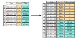
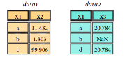
>>> pd.merge(data1, data2, how=' left', on='X1')
>>> pd.merge(data1, data2, how='right', on='X1')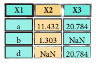
>>> pd.merge(data1, data2, how='inner', on='X1')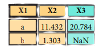
>>> pd.merge(data1, data2, how='outer', on='X1')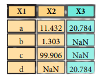
Join
>>> data1.join(data2, how='right')Concatenate
Vertical
>>> s.append(s2)Horizontal/Vertical
>>> pd.concat([s,s2],axis=1, keys=['One','Two'])>>> pd.concat([datal, data2], axis=1, join='inner')Dates
>>> df2['Date']= pd.to_datetime(df2['Date'])>>> df2['Date']= pd.date_range('2000-1-1', periods=6, freq='M')>>>dates= [datetime(2012,5,1), datetime(2012,5,2)]>>>index= pd.Datetimelndex(dates)>>>index= pd.date_range(datetime(2012,2,1), end, freq='BM')Visualization
>>> import matplotlib.pyplot as plt>>> s.plot()>>> plt.show()
>>> df2.plot()>>> plt.show()