Course
Pandas is a popular Python package for data science, and with good reason: it offers powerful, expressive and flexible data structures that make data manipulation and analysis easy, among many other things. The DataFrame is one of these structures.
This tutorial covers pandas DataFrames, from basic manipulations to advanced operations, by tackling 11 of the most popular questions so that you understand -and avoid- the doubts of the Pythonistas who have gone before you.
For more practice, try the first chapter of this Pandas DataFrames course for free!
What are pandas DataFrames?
Before you start, let’s have a brief recap of what DataFrames are.
Those who are familiar with R know the data frame as a way to store data in rectangular grids that can easily be overviewed. Each row of these grids corresponds to measurements or values of an instance, while each column is a vector containing data for a specific variable. This means that a data frame’s rows do not need to contain, but can contain, the same type of values: they can be numeric, character, logical, etc.
Now, DataFrames in Python are very similar: they come with the pandas library, and they are defined as two-dimensional labeled data structures with columns of potentially different types.
In general, you could say that the pandas DataFrame consists of three main components: the data, the index, and the columns.
- Firstly, the DataFrame can contain data that is:
- a Pandas
DataFrame - a Pandas
Series: a one-dimensional labeled array capable of holding any data type with axis labels or index. An example of a Series object is one column from a DataFrame. - a NumPy
ndarray, which can be a record or structured - a two-dimensional
ndarray - dictionaries of one-dimensional
ndarray’s, lists, dictionaries or Series.
Note the difference between np.ndarray and np.array() . The former is an actual data type, while the latter is a function to make arrays from other data structures.
Structured arrays allow users to manipulate the data by named fields: in the example below, a structured array of three tuples is created. The first element of each tuple will be called foo and will be of type int, while the second element will be named bar and will be a float.
Record arrays, on the other hand, expand the properties of structured arrays. They allow users to access fields of structured arrays by attribute rather than by index. You see below that the foo values are accessed in the r2 record array.
An example:
import pandas as pd
import numpy as np

# A structured array
my_array = np.ones(3, dtype=([('foo', int), ('bar', float)]))
# Print the structured array
print(my_array['foo'])

# A record array
my_array2 = my_array.view(np.recarray)
# Print the record array
print(my_array2.foo)
[1 1 1]
[1 1 1]- Besides data, you can also specify the index and column names for your DataFrame. The index, on the one hand, indicates the difference in rows, while the column names indicate the difference in columns. You will see later that these two components of the DataFrame will come in handy when you’re manipulating your data.
If you’re still in doubt about Pandas DataFrames and how they differ from other data structures such as a NumPy array or a Series, you can watch the small presentation below:
Note that in this post, most of the times, the libraries that you need have already been loaded in. The Pandas library is usually imported under the alias pd, while the NumPy library is loaded as np. Remember that when you code in your own data science environment, you shouldn’t forget this import step, which you write just like this:
import numpy as np
import pandas as pd
Now that there is no doubt in your mind about what DataFrames are, what they can do, and how they differ from other structures, it’s time to tackle the most common questions that users have about working with them!
Run and edit the code from this tutorial online
Run code1. How to Create a Pandas DataFrame
Obviously, making your DataFrames is your first step in almost anything that you want to do when it comes to data munging in Python. Sometimes, you will want to start from scratch, but you can also convert other data structures, such as lists or NumPy arrays, to Pandas DataFrames. In this section, you’ll only cover the latter. However, if you want to read more on making empty DataFrames that you can fill up with data later, go to section 7.
Among the many things that can serve as input to make a ‘DataFrame’, a NumPy ndarray is one of them. To make a data frame from a NumPy array, you can just pass it to the DataFrame() function in the data argument.
data = np.array([['','Col1','Col2'],
                ['Row1',1,2],
                ['Row2',3,4]])

print(pd.DataFrame(data=data[1:,1:],
                  index=data[1:,0],
                  columns=data[0,1:]))


    Col1 Col2

Row1    1    2

Row2    3    4
Pay attention to how the code chunks above select elements from the NumPy array to construct the DataFrame: you first select the values that are contained in the lists that start with Row1 and Row2, then you select the index or row numbers Row1 and Row2 and then the column names Col1 and Col2.
Next, you also see that, in the example above, we printed a small selection of the data. This works the same as subsetting 2D NumPy arrays: you first indicate the row that you want to look in for your data, then the column. Don’t forget that the indices start at 0! For data in the example above, you go and look in the rows at index 1 to end, and you select all elements that come after index 1. As a result, you end up selecting 1, 2, 3 and 4.
This approach to making DataFrames will be the same for all the structures that DataFrame() can take on as input.
See the example below:
Remember that the Pandas library has already been imported as pd.
# Take a 2D array as input to your DataFrame
my_2darray = np.array([[1, 2, 3], [4, 5, 6]])
print(pd.DataFrame(my_2darray))

# Take a dictionary as input to your DataFrame
my_dict = {1: ['1', '3'], 2: ['1', '2'], 3: ['2', '4']}
print(pd.DataFrame(my_dict))

# Take a DataFrame as input to your DataFrame
my_df = pd.DataFrame(data=[4,5,6,7], index=range(0,4), columns=['A'])
print(pd.DataFrame(my_df))

# Take a Series as input to your DataFrame
my_series = pd.Series({"Belgium":"Brussels", "India":"New Delhi", "United Kingdom":"London", "United States":"Washington"})
print(pd.DataFrame(my_series))
0 1 2
0 1 2 3
1 4 5 6
1 2 3
0 1 1 2
1 3 2 4
A
0 4
1 5Note that the index of your Series (and DataFrame) contains the keys of the original dictionary, but that they are sorted: Belgium will be the index at 0, while the United States will be the index at 3.
After you have created your DataFrame, you might want to know a little bit more about it. You can use the shape property or the len() function in combination with the .index property:
df = pd.DataFrame(np.array([[1, 2, 3], [4, 5, 6]]))

# Use the `shape` property
print(df.shape)

# Or use the `len()` function with the `index` property
print(len(df))
(2, 3)
2These two options give you slightly different information on your DataFrame: the shape property will provide you with the dimensions of your DataFrame. That means that you will get to know the width and the height of your DataFrame. On the other hand, the len() function, in combination with the index property, will only give you information on the height of your DataFrame.
This all is totally not extraordinary, though, as you explicitly give in the index property.
You could also use df[0].count() to get to know more about the height of your DataFrame, but this will exclude the NaN values (if there are any). That is why calling .count() on your DataFrame is not always the better option.
If you want more information on your DataFrame columns, you can always execute list(my_dataframe.columns.values).
Fundamental DataFrame Operations
Now that you have put your data in a more convenient Pandas DataFrame structure, it’s time to get to the real work!
This first section will guide you through the first steps of working with DataFrames in Python. It will cover the basic operations that you can do on your newly created DataFrame: adding, selecting, deleting, renaming, and more.
2. How to Select an Index or Column from a Pandas DataFrame
Before you start with adding, deleting, and renaming the components of your DataFrame, you first need to know how you can select these elements. So, how do you do this?
Even though you might still remember how to do it from the previous section: selecting an index, column, or value from your DataFrame isn’t that hard, quite the contrary. It’s similar to what you see in other languages (or packages!) that are used for data analysis. If you aren’t convinced, consider the following:
In R, you use the [,] notation to access the data frame’s values.
Now, let’s say you have a DataFrame like this one:
   A  B  C
0  1  2  3
1  4  5  6
2  7  8  9
And you want to access the value that is at index 0, in column ‘A’.
Various options exist to get your value 1 back:
df = pd.DataFrame({"A":[1,4,7], "B":[2,5,8], "C":[3,6,9]})
print(df)
A B C
0 1 2 3
1 4 5 6
2 7 8 9# Using `iloc[]`
print(df.iloc[0][0])
# Using `loc[]`
print(df.loc[0]['A'])
# Using `at[]`
print(df.at[0,'A'])
# Using `iat[]`
print(df.iat[0,0])1
1
1
1The most important ones to remember are, without a doubt, .loc[] and .iloc[]. The subtle differences between these two will be discussed in the next sections.
Enough for now about selecting values from your DataFrame. What about selecting rows and columns? In that case, you would use:
# Use `iloc[]` to select row `0`
print(df.iloc[0])
# Use `loc[]` to select column `'A'`
print(df.loc[:,'A'])A 1
B 2
C 3
Name: 0, dtype: int64
0 1
1 4
2 7
Name: A, dtype: int64For now, it’s enough to know that you can either access the values by calling them by their label or by their position in the index or column. If you don’t see this, look again at the slight differences in the commands: one time, you see [0][0], the other time, you see [0,'A'] to retrieve your value 1.
3. How to Add an Index, Row or Column to a Pandas DataFrame
Now that you have learned how to select a value from a DataFrame, it’s time to get to the real work and add an index, row or column to it!
Adding an Indext to a DataFrame
When you create a DataFrame, you have the option to add input to the ‘index’ argument to make sure that you have the index that you desire. When you don’t specify this, your DataFrame will have, by default, a numerically valued index that starts with 0 and continues until the last row of your DataFrame.
However, even when your index is specified for you automatically, you still have the power to re-use one of your columns and make it your index. You can easily do this by calling set_index() on your DataFrame. Try this out below!
# Print out your DataFrame `df` to check it out
print(df)
# Set 'C' as the index of your DataFrame
df.set_index('C') A B C
0 1 2 3
1 4 5 6
2 7 8 9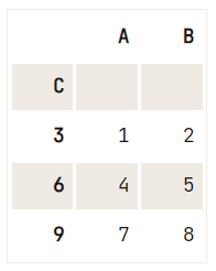
Adding Rows to a DataFrame
Before you can get to the solution, it’s first a good idea to grasp the concept of loc and how it differs from other indexing attributes such as .iloc[] and .ix[]:
- .loc[] works on labels of your index. This means that if you give in loc[2], you look for the values of your DataFrame that have an index labeled 2.
- .iloc[] works on the positions in your index. This means that if you give in iloc[2], you look for the values of your DataFrame that are at index ’2`.
- .ix[] is a more complex case: when the index is integer-based, you pass a label to .ix[]. ix[2] then means that you’re looking in your DataFrame for values that have an index labeled 2. This is just like .loc[]! However, if your index is not solely integer-based, ix will work with positions, just like .iloc[].
This all might seem very complicated. Let’s illustrate all of this with a small example:
df = pd.DataFrame(data=np.array([[1, 2, 3], [4, 5, 6], [7, 8, 9]]), index= [2, 'A', 4], columns=[48, 49, 50])
# Pass `2` to `loc`
print(df.loc[2])
# Pass `2` to `iloc`
print(df.iloc[2])48 1
49 2
50 3
Name: 2, dtype: int64
48 7
49 8
50 9
Name: 4, dtype: int64Note that in this case, you used an example of a DataFrame that is not solely integer-based as to make it easier for you to understand the differences. You clearly see that passing 2 to .loc[] or .iloc[]/.ix[] does not give back the same result!
- You know that .loc[] will go and look at the values that are at label 2. The result that you get back will be
48 1
49 2
50 3- You also know that
.iloc[]will go and look at the positions in the index. When you pass2, you will get back:
48 7
49 8
50 9- Since the index doesn’t only contain integers,
.ix[]will have the same behavior asilocand look at the positions in the index. You will get back the same result as.iloc[].
Now that the difference between .iloc[], .loc[] and .ix[] is clear, you are ready to give adding rows to your DataFrame a go!
Tip: as a consequence of what you have just read, you understand now also that the general recommendation is that you use .loc to insert rows in your DataFrame. That is because if you would use df.ix[], you might try to reference a numerically valued index with the index value and accidentally overwrite an existing row of your DataFrame. You should avoid this!
Check out the difference once more in the DataFrame below:
df = pd.DataFrame(data=np.array([[1, 2, 3], [4, 5, 6], [7, 8, 9]]), index= [2.5, 12.6, 4.8], columns=[48, 49, 50])
# This will make an index labeled `2` and add the new values
df.loc[2] = [11, 12, 13]
print(df) 48 49 50
2.5 1 2 3
12.6 4 5 6
4.8 7 8 9
2.0 11 12 13You can see why all of this can be confusing, right?
Adding a Column to your DataFrame
In some cases, you want to make your index part of your DataFrame. You can easily do this by taking a column from your DataFrame or by referring to a column that you haven’t made yet and assigning it to the .index property, just like this:
df = pd.DataFrame(data=np.array([[1, 2, 3], [4, 5, 6], [7, 8, 9]]), columns=['A', 'B', 'C'])
# Use `.index`
df['D'] = df.index
# Print `df`
print(df) A B C D
0 1 2 3 0
1 4 5 6 1
2 7 8 9 2In other words, you tell your DataFrame that it should take column A as its index.
However, if you want to append columns to your DataFrame, you could also follow the same approach as when you would add an index to your DataFrame: you use .loc[] or .iloc[]. In this case, you add a Series to an existing DataFrame with the help of .loc[]:
# Study the DataFrame `df`
print(df)
# Append a column to `df`
df.loc[:, 4] = pd.Series(['5', '6', '7'], index=df.index)
# Print out `df` again to see the changes
print(df) A B C D
0 1 2 3 0
1 4 5 6 1
2 7 8 9 2
A B C D 4
0 1 2 3 0 5
1 4 5 6 1 6
2 7 8 9 2 7Remember a Series object is much like a column of a DataFrame. That explains why you can easily add a Series to an existing DataFrame. Note also that the observation that was made earlier about .loc[] still stays valid, even when you’re adding columns to your DataFrame!
Resetting the Index of your DataFrame
When your index doesn’t look entirely the way you want it to, you can opt to reset it. You can easily do this with .reset_index(). However, you should still watch out, as you can pass several arguments that can make or break the success of your reset:
# Check out the weird index of your dataframe
print(df)
# Use `reset_index()` to reset the values.
df_reset = df.reset_index(level=0, drop=True)
# Print `df_reset`
print(df_reset) A B C D 4
0 1 2 3 0 5
1 4 5 6 1 6
2 7 8 9 2 7
A B C D 4
0 1 2 3 0 5
1 4 5 6 1 6
2 7 8 9 2 7You can try replacing the drop argument by inplace in the example above and see what happens!
Note how you use the drop argument to indicate that you want to get rid of the index that was there. If you would have used inplace, the original index with floats is added as an extra column to your DataFrame.
4. How to Delete Indices, Rows or Columns from a Pandas Data Frame
Now that you have seen how to select and add indices, rows, and columns to your DataFrame, it’s time to consider another use case: removing these three from your data structure.
Deleting an Index from your DataFrame
If you want to remove the index from your DataFrame, you should reconsider because DataFrames and Series always have an index.
However, what you *can* do is, for example:
- resetting the index of your DataFrame (go back to the previous section to see how it is done) or
- remove the index name, if there is any, by executing
del df.index.name, - remove duplicate index values by resetting the index, dropping the duplicates of the index column that has been added to your DataFrame and reinstating that duplicateless column again as the index
- and lastly, remove an index, and with it a row. This is elaborated further on in this tutorial.
df = pd.DataFrame(data=np.array([[1, 2, 3], [4, 5, 6], [7, 8, 9], [40, 50, 60], [23, 35, 37]]),
index= [2.5, 12.6, 4.8, 4.8, 2.5],
columns=[48, 49, 50])
df.reset_index().drop_duplicates(subset='index', keep='last').set_index('index')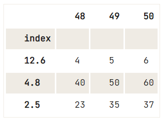
Now that you know how to remove an index from your DataFrame, you can go on to removing columns and rows!
Deleting a Column from your DataFrame
To get rid of (a selection of) columns from your DataFrame, you can use the drop() method:
df = pd.DataFrame(data=np.array([[1, 2, 3], [4, 5, 6], [7, 8, 9]]), columns=['A', 'B', 'C'])
# Check out the DataFrame `df`
print(df)
# Drop the column with label 'A'
df.drop('A', axis=1, inplace=True)
# Drop the column at position 1
df.drop(df.columns[[1]], axis=1) A B C
0 1 2 3
1 4 5 6
2 7 8 9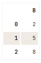
You might think now: well, this is not so straightforward; There are some extra arguments that are passed to the drop() method!
- The
axisargument is either 0 when it indicates rows and 1 when it is used to drop columns. - You can set
inplaceto True to delete the column without having to reassign the DataFrame.
Removing a Row from your DataFrame
You can remove duplicate rows from your DataFrame by executing df.drop_duplicates(). You can also remove rows from your DataFrame, taking into account only the duplicate values that exist in one column.
Check out this example:
df = pd.DataFrame(data=np.array([[1, 2, 3], [4, 5, 6], [7, 8, 9], [40, 50, 60], [23, 35, 37]]),
index= [2.5, 12.6, 4.8, 4.8, 2.5],
columns=[48, 49, 50])
# Check out your DataFrame `df`
print(df)
# Drop the duplicates in `df`
df.drop_duplicates([48], keep='last') 48 49 50
2.5 1 2 3
12.6 4 5 6
4.8 7 8 9
4.8 40 50 60
2.5 23 35 37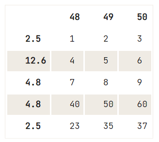
If there is no uniqueness criterion to the deletion that you want to perform, you can use the drop() method, where you use the index property to specify the index of which rows you want to remove from your DataFrame:
# Check out the DataFrame `df`
print(df)
# Drop the index at position 1
df.drop(df.index[1]) 48 49 50
2.5 1 2 3
12.6 4 5 6
4.8 7 8 9
4.8 40 50 60
2.5 23 35 37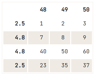
After this command, you might want to reset the index again.
Tip: try resetting the index of the resulting DataFrame for yourself! Don’t forget to use the drop argument if you deem it necessary.
5. How to Rename the Index or Columns of a Pandas DataFrame
To give the columns or your index values of your dataframe a different value, it’s best to use the .rename() method.
df = pd.DataFrame(data=np.array([[1, 2, 3], [4, 5, 6], [7, 8, 9]]), columns=['A', 'B', 'C'])
# Check out your DataFrame `df`
print(df)
# Define the new names of your columns
newcols = {
'A': 'new_column_1',
'B': 'new_column_2',
'C': 'new_column_3'
}
# Use `rename()` to rename your columns
df.rename(columns=newcols, inplace=True)
# Rename your index
df.rename(index={1: 'a'}) A B C
0 1 2 3
1 4 5 6
2 7 8 9
Tip: try changing the inplace argument in the first task (renaming your columns) to False and see what the script now renders as a result. You see that now the DataFrame hasn’t been reassigned when renaming the columns. As a result, the second task takes the original DataFrame as input and not the one that you just got back from the first rename() operation.
Beyond the Pandas DataFrame Basics
Now that you have gone through a first set of questions about Pandas’ DataFrames, it’s time to go beyond the basics and get your hands dirty for real because there is far more to DataFrames than what you have seen in the first section.
6. How To Format The Data in Your Pandas DataFrame
Most of the time, you will also want to be able to do some operations on the actual values that are contained within your DataFrame. In the following sections, you’ll cover several ways in which you can format your pandas DataFrame’s values
Replacing all Occurrences of a String in a DataFrame
To replace certain strings in your DataFrame, you can easily use replace(): pass the values that you would like to change, followed by the values you want to replace them by.
Just like this:
df = pd.DataFrame({"Student1":['OK','Awful','Acceptable'],
"Student2":['Perfect','Awful','OK'],
"Student3":['Acceptable','Perfect','Poor']})
# Study the DataFrame `df` first
print(df)
# Replace the strings by numerical values (0-4)
df.replace(['Awful', 'Poor', 'OK', 'Acceptable', 'Perfect'], [0, 1, 2, 3, 4]) Student1 Student2 Student3
0 OK Perfect Acceptable
1 Awful Awful Perfect
2 Acceptable OK Poor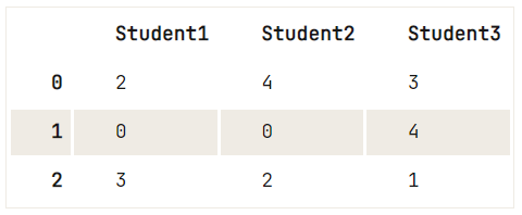
Note that there is also a regex argument that can help you out tremendously when you’re faced with strange string combinations:
df = pd.DataFrame([["1\n", 2, "3\n"], [4, 5, "6\n"] ,[7, "8\n", 9]])
# Check out your DataFrame `df`
print(df)
# Replace strings by others with `regex`
df.replace({'\n': ''}, regex=True) 0 1 2
0 1\n 2 3\n
1 4 5 6\n
2 7 8\n 9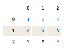
In short, replace() is mostly what you need to deal with when you want to replace values or strings in your DataFrame by others!
Removing Parts from Strings in the Cells of your DataFrame
Removing unwanted parts of strings is cumbersome work. Luckily, there is an easy solution to this problem!
df = pd.DataFrame([["+-1aAbBcC", "2", "+-3aAbBcC"], ["4", "5", "+-6aAbBcC"] ,["7", "+-8aAbBcC", "9"]])
# Check out your DataFrame
print(df)
# Delete unwanted parts from the strings in the first column
df[0] = df[0].map(lambda x: x.lstrip('+-').rstrip('aAbBcC'))
# Check out the result again
df 0 1 2
0 +-1aAbBcC 2 +-3aAbBcC
1 4 5 +-6aAbBcC
2 7 +-8aAbBcC 9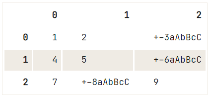
You use map() on the column result to apply the lambda function over each element or element-wise of the column. The function in itself takes the string value and strips the + or - that’s located on the left, and also strips away any of the six aAbBcC on the right.
Splitting Text in a Column into Multiple Rows in a DataFrame
This is somewhat a more difficult formatting task. However, the next code chunk will walk you through the steps:
df = pd.DataFrame({"Age": [34, 22, 19],
"PlusOne":[0,0,1],
"Ticket":["23:44:55", "66:77:88", "43:68:05 56:34:12"]})
# Inspect your DataFrame `df`
print(df)
# Split out the two values in the third row
# Make it a Series
# Stack the values
ticket_series = df['Ticket'].str.split(' ').apply(pd.Series, 1).stack()
# Get rid of the stack:
# Drop the level to line up with the DataFrame
ticket_series.index = ticket_series.index.droplevel(-1)
print(ticket_series) Age PlusOne Ticket
0 34 0 23:44:55
1 22 0 66:77:88
2 19 1 43:68:05 56:34:12
0 23:44:55
1 66:77:88
2 43:68:05
2 56:34:12
dtype: object
0
0 23:44:55
1 66:77:88
2 43:68:05
2 56:34:12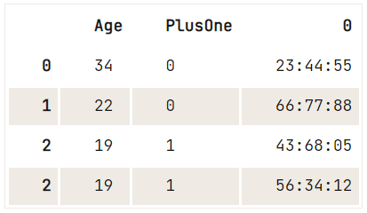
In short, what you do is:
- First, you inspect the DataFrame at hand. You see that the values in the last row and in the last column are a bit too long. It appears there are two tickets because a guest has taken a plus-one to the concert.
- You take the
Ticketcolumn from the DataFramedfand strings on a space. This will make sure that the two tickets will end up in two separate rows in the end. Next, you take these four values (the four ticket numbers) and put them into a Series object:
0 1
0 23:44:55 NaN
1 66:77:88 NaN
2 43:68:05 56:34:12- That still doesn’t seem quite right. You have
NaNvalues in there! You have to stack the Series to make sure you don’t have anyNaNvalues in the resulting Series. - Next, you see that your Series is stacked.
0 0 23:44:55
1 0 66:77:88
2 0 43:68:05
1 56:34:12- That is not ideal either. That is why you drop the level to line up with the DataFrame:
0 23:44:55
1 66:77:88
2 43:68:05
2 56:34:12
dtype: object- That is what you’re looking for.
- Transform your Series to a DataFrame to make sure you can join it back to your initial DataFrame. However, to avoid having any duplicates in your DataFrame, you can delete the original
Ticketcolumn.
Applying a Function to your Pandas DataFrame’s Columns or Rows
You might want to adjust the data in your DataFrame by applying a function to it. Let’s begin answering this question by making your own lambda function:
doubler = lambda x: x*2Tip: if you want to know more about functions in Python, consider taking this Python functions tutorial.
df = pd.DataFrame(data=np.array([[1, 2, 3], [4, 5, 6], [7, 8, 9]]), columns=['A', 'B', 'C'])
# Study the `df` DataFrame
print(df)
# Apply the `doubler` function to the `A` DataFrame column
df['A'].apply(doubler)
  A  B  C

0  1  2  3

1  4  5  6

2  7  8  9
0 2
1 8
2 14
Name: A, dtype: int64Note that you can also select the row of your DataFrame and apply the doubler lambda function to it. Remember that you can easily select a row from your DataFrame by using .loc[] or .iloc[].
Then, you would execute something like this, depending on whether you want to select your index based on its position or based on its label:
df.loc[0].apply(doubler)Note that the apply() function only applies the doubler function along the axis of your DataFrame. That means that you target either the index or the columns. Or, in other words, either a row or a column.
However, if you want to apply it to each element or element-wise, you can make use of the map() function. You can just replace the apply() function in the code chunk above with map(). Don’t forget to still pass the doubler function to it to make sure you multiply the values by 2.
Let’s say you want to apply this doubling function not only to the A column of your DataFrame but to the whole of it. In this case, you can use applymap() to apply the doubler function to every single element in the entire DataFrame:
doubled_df = df.applymap(doubler)
print(doubled_df)
A B C
0 2 4 6
1 8 10 12
2 14 16 18Note that in these cases, we have been working with lambda functions or anonymous functions that get created at runtime. However, you can also write your own function. For example:
def doubler(x):
    if x % 2 == 0:
        return x
    else:
        return x * 2

# Use `applymap()` to apply `doubler()` to your DataFrame
doubled_df = df.applymap(doubler)

# Check the DataFrame
print(doubled_df)
A B C
0 2 2 6
1 4 10 6
2 14 8 18If you want more information on the flow of control in Python, you can always check out our other resources.
7. How to Create an Empty DataFrame
The function that you will use is the Pandas Dataframe() function: it requires you to pass the data that you want to put in, the indices and the columns.
Remember that the data that is contained within the data frame doesn’t have to be homogenous. It can be of different data types!
There are several ways in which you can use this function to make an empty DataFrame. Firstly, you can use numpy.nan to initialize your data frame with NaNs. Note that numpy.nan has type float.
df = pd.DataFrame(np.nan, index=[0,1,2,3], columns=['A'])
print(df)
A
0 NaN
1 NaN
2 NaN
3 NaNRight now, the data type of the data frame is inferred by default: because numpy.nan has type float, the data frame will also contain values of type float. You can, however, also force the DataFrame to be of a particular type by adding the attribute dtype and filling in the desired type. Just like in this example:
df = pd.DataFrame(index=range(0,4),columns=['A'], dtype='float')
print(df)
   A

0 NaN

1 NaN

2 NaN

3 NaNNote that if you don’t specify the axis labels or index, they will be constructed from the input data based on common sense rules.
8. Does Pandas Recognize Dates when Importing Data?
Pandas can recognize it, but you need to help it a tiny bit: add the argument parse_dates when you’reading in data from, let’s say, a comma-separated value (CSV) file:
import pandas as pd
pd.read_csv('yourFile', parse_dates=True)

# or this option:
pd.read_csv('yourFile', parse_dates=['columnName'])
There are, however, always weird date-time formats.
No worries! In such cases, you can construct your own parser to deal with this. You could, for example, make a lambda function that takes your DateTime and controls it with a format string.
import pandas as pd
dateparser = lambda x: pd.datetime.strptime(x, '%Y-%m-%d %H:%M:%S')

# Which makes your read command:
pd.read_csv(infile, parse_dates=['columnName'], date_parser=dateparse)

# Or combine two columns into a single DateTime column
pd.read_csv(infile, parse_dates={'datetime': ['date', 'time']}, date_parser=dateparse)
9. When, why, and how you Should Reshape your Pandas DataFrame
Reshaping your DataFrame is transforming it so that the resulting structure makes it more suitable for your data analysis. In other words, reshaping is not so much concerned with formatting the values that are contained within the DataFrame, but more about transforming the shape of it.
This answers the when and why. But how would you reshape your DataFrame?
There are three ways of reshaping that frequently raise questions with users: pivoting, stacking and unstacking and melting.
Pivotting your DataFrame
You can use the pivot() function to create a new derived table out of your original one. When you use the function, you can pass three arguments:
values: this argument allows you to specify which values of your original DataFrame you want to see in your pivot table.columns: whatever you pass to this argument will become a column in your resulting table.index: whatever you pass to this argument will become an index in your resulting table.
# Import pandas
import pandas as pd

# Create your DataFrame
products = pd.DataFrame({'category': ['Cleaning', 'Cleaning', 'Entertainment', 'Entertainment', 'Tech', 'Tech'],
        'store': ['Walmart', 'Dia', 'Walmart', 'Fnac', 'Dia','Walmart'],
        'price':[11.42, 23.50, 19.99, 15.95, 55.75, 111.55],
        'testscore': [4, 3, 5, 7, 5, 8]})

# Use `pivot()` to pivot the DataFrame
pivot_products = products.pivot(index='category', columns='store', values='price')

# Check out the result
print(pivot_products)
store Dia Fnac Walmart
category
Cleaning 23.50 NaN 11.42
Entertainment NaN 15.95 19.99
Tech 55.75 NaN 111.55When you don’t specifically fill in what values you expect to be present in your resulting table, you will pivot by multiple columns:
# Import the Pandas library
import pandas as pd
# Construct the DataFrame
products = pd.DataFrame({'category': ['Cleaning', 'Cleaning', 'Entertainment', 'Entertainment', 'Tech', 'Tech'],
'store': ['Walmart', 'Dia', 'Walmart', 'Fnac', 'Dia','Walmart'],
'price':[11.42, 23.50, 19.99, 15.95, 55.75, 111.55],
'testscore': [4, 3, 5, 7, 5, 8]})
# Use `pivot()` to pivot your DataFrame
pivot_products = products.pivot(index='category', columns='store')
# Check out the results
print(pivot_products)
             price                testscore

store            Dia   Fnac Walmart       Dia Fnac Walmart

category

Cleaning       23.50    NaN   11.42       3.0  NaN     4.0

Entertainment    NaN  15.95   19.99       NaN  7.0     5.0

Tech           55.75    NaN  111.55       5.0  NaN     8.0
Note that your data can not have rows with duplicate values for the columns that you specify. If this is not the case, you will get an error message. If you can’t ensure the uniqueness of your data, you will want to use the pivot_table method instead:
# Import the Pandas library
import pandas as pd

# Your DataFrame
products = pd.DataFrame({'category': ['Cleaning', 'Cleaning', 'Entertainment', 'Entertainment', 'Tech', 'Tech'],
                        'store': ['Walmart', 'Dia', 'Walmart', 'Fnac', 'Dia','Walmart'],
                        'price':[11.42, 23.50, 19.99, 15.95, 19.99, 111.55],
                        'testscore': [4, 3, 5, 7, 5, 8]})

# Pivot your `products` DataFrame with `pivot_table()`
pivot_products = products.pivot_table(index='category', columns='store', values='price', aggfunc='mean')

# Check out the results
print(pivot_products)
store Dia Fnac Walmart
category
Cleaning 23.50 NaN 11.42
Entertainment NaN 15.95 19.99
Tech 19.99 NaN 111.55Note the additional argument aggfunc that gets passed to the pivot_table method. This argument indicates that you use an aggregation function used to combine multiple values. In this example, you can clearly see that the mean function is used.
Using stack() and unstack() to Reshape your Pandas DataFrame
You have already seen an example of stacking in section 5. In essence, you might still remember that when you stack a DataFrame, you make it taller. You move the innermost column index to become the innermost row index. You return a DataFrame with an index with a new inner-most level of row labels.
Go back to the full walk-through in section 5 if you’re unsure of the workings ofstack().
The inverse of stacking is called unstacking. Much like stack(), you use unstack() to move the innermost row index to become the innermost column index.
For an explanation of pands pivoting, stacking and unstacking, check out our Reshaping Data with pandas course.
Reshape your DataFrame With melt()
Melting is considered useful in cases where you have data that has one or more columns that are identifier variables, while all other columns are considered measured variables.
These measured variables are all “unpivoted” to the row axis. That is, while the measured variables that were spread out over the width of the DataFrame, the melt will make sure that they will be placed in the height of it. Or, yet in other words, your DataFrame will now become longer instead of wider.
As a result, you have two non-identifier columns, namely, ‘variable’ and ‘value’.
Let’s illustrate this with an example:
# The `people` DataFrame
people = pd.DataFrame({'FirstName' : ['John', 'Jane'],
                       'LastName' : ['Doe', 'Austen'],
                       'BloodType' : ['A-', 'B+'],
                       'Weight' : [90, 64]})

# Use `melt()` on the `people` DataFrame
print(pd.melt(people, id_vars=['FirstName', 'LastName'], var_name='measurements'))
FirstName LastName measurements value
0 John Doe BloodType A-
1 Jane Austen BloodType B+
2 John Doe Weight 90
3 Jane Austen Weight 64If you’re looking for more ways to reshape your data, check out the documentation.
10. How to Iterate over a Pandas DataFrame
You can iterate over the rows of your DataFrame with the help of a for loop in combination with an iterrows() call on your DataFrame:
df = pd.DataFrame(data=np.array([[1, 2, 3], [4, 5, 6], [7, 8, 9]]), columns=['A', 'B', 'C'])

for index, row in df.iterrows() :
    print(row['A'], row['B'])
1 2
4 5
7 8iterrows() allows you to efficiently loop over your DataFrame rows as (index, Series) pairs. In other words, it gives you (index, row) tuples as a result.
11. How to Write a Pandas DataFrame to a File
When you have done your data munging and manipulation with Pandas, you might want to export the DataFrame to another format. This section will cover two ways of outputting your pandas DataFrame to a CSV or to an Excel file.
Output a DataFrame to CSV
To write a DataFrame as a CSV file, you can use to_csv():
import pandas as pd
df.to_csv('myDataFrame.csv')
That piece of code seems quite simple, but this is just where the difficulties begin for most people because you will have specific requirements for the output of your data. Maybe you don’t want a comma as a delimiter, or you want to specify a specific encoding.
Don’t worry! You can pass some additional arguments to to_csv() to make sure that your data is outputted the way you want it to be!
- To delimit by a tab, use the
separgument:
import pandas as pd
df.to_csv('myDataFrame.csv', sep='\t')- To use a specific character encoding, you can use the
encodingargument:
import pandas as pd
df.to_csv('myDataFrame.csv', sep='\t', encoding='utf-8')- Furthermore, you can specify how you want your
NaNor missing values to be represented, whether or not you want to output the header, whether or not you want to write out the row names, whether you want compression, you can read up on the options.
Writing a DataFrame to Excel
Similarly to what you did to output your DataFrame to CSV, you can use to_excel() to write your table to Excel. However, it is a bit more complicated:
import pandas as pd
writer = pd.ExcelWriter('myDataFrame.xlsx')
df.to_excel(writer, 'DataFrame')
writer.save()
Note, however, that, just like with to_csv(), you have a lot of extra arguments such as startcol, startrow, and so on, to make sure you output your data correctly. You can learn more about how to import data from and export data to CSV files using pandas in our tutorial.
If, however, you want more information on IO tools in Pandas, you check out the pandas DataFrames to excel documentation.
Python for Data Science is more than DataFrames
That’s it! You've successfully completed the Pandas DataFrame tutorial!
The answers to the 11 frequently asked Pandas questions represent essential functions that you will need to import, clean, and manipulate your data for your data science work. Are you not sure that you have gone deep enough into this matter? Our Importing Data In Python course will help you out! If you’ve got the hang out of this, you might want to see Pandas at work in a real-life project. The Importance of Preprocessing in Data Science and the Machine Learning Pipeline tutorial series is a must-read, and the open course Introduction to Python & Machine Learning is a must-complete.

