Matplotlib Cheat Sheet: Plotting in Python

Data visualization and storytelling with your data are essential skills that every data scientist needs to communicate insights gained from analyses effectively to any audience out there. 

For most beginners, the first package that they use to get in touch with data visualization and storytelling is, naturally, Matplotlib: it is a Python 2D plotting library that enables users to make publication-quality figures. But, what might be even more convincing is the fact that other packages, such as Pandas, intend to build more plotting integration with Matplotlib as time goes on.

However, what might slow down beginners is the fact that this package is pretty extensive. There is so much that you can do with it and it might be hard to still keep a structure when you're learning how to work with Matplotlib.   

DataCamp has created a Matplotlib cheat sheet for those who might already know how to use the package to their advantage to make beautiful plots in Python, but that still want to keep a one-page reference handy. Of course, for those who don't know how to work with Matplotlib, this might be the extra push be convinced and to finally get started with data visualization in Python. 

(By the way, if you want to get started with this Python package, you might want to consider our Matplotlib tutorial.)

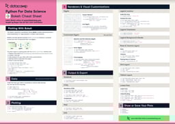
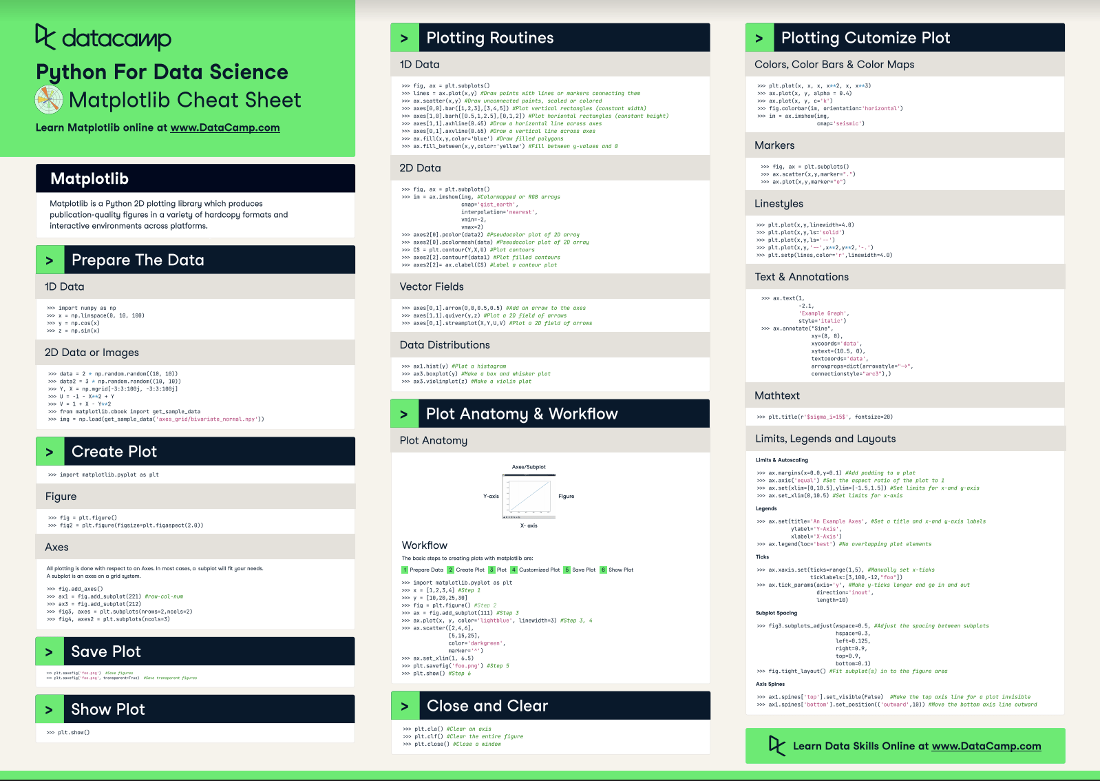
You'll see that this cheat sheet presents you with the six basic steps that you can go through to make beautiful plots. 

Check out the infographic by clicking on the button below:

With this handy reference, you'll familiarize yourself in no time with the basics of Matplotlib: you'll learn how you can prepare your data, create a new plot, use some basic plotting routines to your advantage, add customizations to your plots, and save, show and close the plots that you make.

What might have looked difficult before will definitely be more clear once you start using this cheat sheet! Use it in combination with the Matplotlib Gallery, the documentation and our tutorial.   

Also, don't miss out on our other cheat sheets for data science that cover SciPy, Numpy, Scikit-Learn, Bokeh, Pandas and the Python basics.

Matplotlib 

Matplotlib is a Python 2D plotting library which produces publication-quality figures in a variety of hardcopy formats and interactive environments across platforms.

Prepare the Data 

1D Data 

>>> import numpy as np
>>> x = np.linspace(0, 10, 100)
>>> y = np.cos(x)
>>> z = np.sin(x)

2D Data or Images 

>>> data = 2 * np.random.random((10, 10))
>>> data2 = 3 * np.random.random((10, 10))
>>> Y, X = np.mgrid[-3:3:100j, -3:3:100j]
>>> U = 1 X** 2 + Y
>>> V = 1 + X Y**2
>>> from matplotlib.cbook import get_sample_data
>>> img = np.load(get_sample_data('axes_grid/bivariate_normal.npy'))

Create Plot

>>> import matplotlib.pyplot as plt

Figure 

>>> fig = plt.figure()
>>> fig2 = plt.figure(figsize=plt.figaspect(2.0))

Axes 

>>> fig.add_axes()
>>> ax1 = fig.add_subplot(221) #row-col-num
>>> ax3 = fig.add_subplot(212)
>>> fig3, axes = plt.subplots(nrows=2,ncols=2)
>>> fig4, axes2 = plt.subplots(ncols=3)

Save Plot 

>>> plt.savefig('foo.png') #Save figures
>>> plt.savefig('foo.png',  transparent=True) #Save transparent figures

Show Plot

>>> plt.show()

Plotting Routines 

1D Data 

>>> fig, ax = plt.subplots()
>>> lines = ax.plot(x,y) #Draw points with lines or markers connecting them
>>> ax.scatter(x,y) #Draw unconnected points, scaled or colored
>>> axes[0,0].bar([1,2,3],[3,4,5]) #Plot vertical rectangles (constant width)
>>> axes[1,0].barh([0.5,1,2.5],[0,1,2]) #Plot horiontal rectangles (constant height)
>>> axes[1,1].axhline(0.45) #Draw a horizontal line across axes
>>> axes[0,1].axvline(0.65) #Draw a vertical line across axes
>>> ax.fill(x,y,color='blue') #Draw filled polygons
>>> ax.fill_between(x,y,color='yellow') #Fill between y values and 0

2D Data 

>>> fig, ax = plt.subplots()
>>> im = ax.imshow(img, #Colormapped or RGB arrays
      cmap= 'gist_earth', 
      interpolation= 'nearest',
      vmin=-2,
      vmax=2)
>>> axes2[0].pcolor(data2) #Pseudocolor plot of 2D array
>>> axes2[0].pcolormesh(data) #Pseudocolor plot of 2D array
>>> CS = plt.contour(Y,X,U) #Plot contours
>>> axes2[2].contourf(data1) #Plot filled contours
>>> axes2[2]= ax.clabel(CS) #Label a contour plot

Vector Fields 

>>> axes[0,1].arrow(0,0,0.5,0.5) #Add an arrow to the axes
>>> axes[1,1].quiver(y,z) #Plot a 2D field of arrows
>>> axes[0,1].streamplot(X,Y,U,V) #Plot a 2D field of arrows

Data Distributions 

>>> ax1.hist(y) #Plot a histogram
>>> ax3.boxplot(y) #Make a box and whisker plot
>>> ax3.violinplot(z)  #Make a violin plot

Plot Anatomy & Workflow 

Plot Anatomy 

 y-axis      

                           x-axis 

Workflow 

The basic steps to creating plots with matplotlib are:

1 Prepare Data
2 Create Plot
3 Plot
4 Customized Plot
5 Save Plot
6 Show Plot

>>> import matplotlib.pyplot as plt
>>> x = [1,2,3,4]  #Step 1
>>> y = [10,20,25,30] 
>>> fig = plt.figure() #Step 2
>>> ax = fig.add_subplot(111) #Step 3
>>> ax.plot(x, y, color= 'lightblue', linewidth=3)  #Step 3, 4
>>> ax.scatter([2,4,6],
          [5,15,25],
          color= 'darkgreen',
          marker= '^' )
>>> ax.set_xlim(1, 6.5)
>>> plt.savefig('foo.png' ) #Step 5
>>> plt.show() #Step 6

Close and Clear 

>>> plt.cla()  #Clear an axis
>>> plt.clf(). #Clear the entire figure
>>> plt.close(). #Close a window

Plotting Customize Plot 

Colors, Color Bars & Color Maps 

>>> plt.plot(x, x, x, x**2, x, x** 3)
>>> ax.plot(x, y, alpha = 0.4)
>>> ax.plot(x, y, c= 'k')
>>> fig.colorbar(im, orientation= 'horizontal')
>>> im = ax.imshow(img,
            cmap= 'seismic' )

Markers 

>>> fig, ax = plt.subplots()
>>> ax.scatter(x,y,marker= ".")
>>> ax.plot(x,y,marker= "o")

Linestyles 

>>> plt.plot(x,y,linewidth=4.0)
>>> plt.plot(x,y,ls= 'solid') 
>>> plt.plot(x,y,ls= '--') 
>>> plt.plot(x,y,'--' ,x**2,y**2,'-.' ) 
>>> plt.setp(lines,color= 'r',linewidth=4.0)

Text & Annotations 

>>> ax.text(1,
           -2.1, 
           'Example Graph', 
            style= 'italic' )
>>> ax.annotate("Sine", 
xy=(8, 0),
xycoords= 'data', 
xytext=(10.5, 0),
textcoords= 'data', 
arrowprops=dict(arrowstyle= "->", 
connectionstyle="arc3"),)

Mathtext 

>>> plt.title(r '$sigma_i=15$', fontsize=20)

Limits, Legends and Layouts 

Limits & Autoscaling 

>>> ax.margins(x=0.0,y=0.1) #Add padding to a plot
>>> ax.axis('equal')  #Set the aspect ratio of the plot to 1
>>> ax.set(xlim=[0,10.5],ylim=[-1.5,1.5])  #Set limits for x-and y-axis
>>> ax.set_xlim(0,10.5) #Set limits for x-axis

Legends 

>>> ax.set(title= 'An Example Axes',  #Set a title and x-and y-axis labels
            ylabel= 'Y-Axis', 
            xlabel= 'X-Axis')
>>> ax.legend(loc= 'best')  #No overlapping plot elements

Ticks 

>>> ax.xaxis.set(ticks=range(1,5),  #Manually set x-ticks
             ticklabels=[3,100, 12,"foo" ])
>>> ax.tick_params(axis= 'y', #Make y-ticks longer and go in and out
             direction= 'inout', 
              length=10)

Subplot Spacing 

>>> fig3.subplots_adjust(wspace=0.5,   #Adjust the spacing between subplots
             hspace=0.3,
             left=0.125,
             right=0.9,
             top=0.9,
             bottom=0.1)
>>> fig.tight_layout() #Fit subplot(s) in to the figure area

Axis Spines 

>>> ax1.spines[ 'top'].set_visible(False) #Make the top axis line for a plot invisible
>>> ax1.spines['bottom' ].set_position(( 'outward',10))  #Move the bottom axis line outward