Curso
Welcome to the world of DynamoDB, where efficiency and unlimited scalability converge into a single table. In this comprehensive tutorial, we'll embark on an empowering journey, unveiling the true potential of NoSQL single table database design.
Discover the art of simplifying complex data models while harnessing the full power of a unified structure capable of effortlessly accommodating your ever-expanding needs.
Whether you're a seasoned developer well-versed in NoSQL databases or just starting your database journey, get ready to unlock a new level of scalability for your applications with a powerful data architecture!
What is NoSQL?
Before we begin, it is important to understand the difference between NoSQL and the relational database, under what scenarios we would use each, and why these technologies were invented. This requires a brief look at the history of data processing.
You can read more about the importance of NoSQL databases in data science in a separate blog post.
Relational databases
The relational database is a well-known, widely used technology that has been around since the 1970s. Two of the main problems the relational database solves are storage and referential integrity.
The data is “normalized,” typically to 3rd normal form, which reduces the size of the data footprint whilst also ensuring that any updates to the data remain consistent with the rest of the data.
The size of the persisted data footprint was crucial because, historically, the most expensive component in the data center was the hard drive. This is no longer the case today as it is now the CPU that is most expensive, and data storage has drastically reduced in cost. This doesn’t mean the relational database is obsolete; it has valid applications for:
- OLAP
- Data warehouses
- Ad hoc queries
- Applications where the access patterns are not well-defined
- CMS / headless CMS
NoSQL databases
Data pressure is the ability of a system to process a given amount of data within reasonable cost and/or time.
NoSQL databases were invented in the late 1990s to address data pressure issues affecting relational database performance due to ever-increasing volumes of application data.
The CPU in a relational database can be thought of as one of the main bottlenecks as the relational database server strains to fetch and stitch together normalized data into the denormalized views that applications generally consume.
This can be alleviated by adding read replica servers, but NoSQL takes a different approach and stores application data in a denormalized form ready for applications to consume. This means the data footprint is larger than that of a relational database but lightens the load on the CPU, effectively making the database server just a simple router that uses a hash algorithm to point to a location on a hard disk in the data center. Typical usages for NoSQL databases are:
- OLTP
- Applications with well-known access patterns
- Applications that need to scale horizontally to support large regional or global volumes of demand
Numerous studies have provided us with enough objective data on this topic to present a graph representing the performance of SQL vs NoSQL at scale.
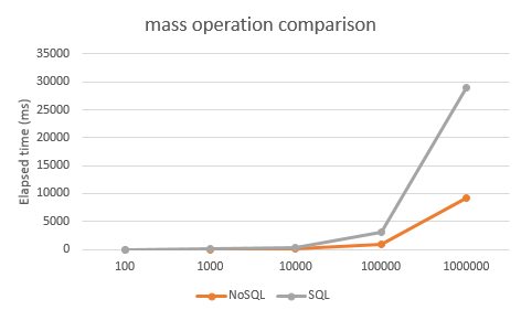
The last point to make clear is that the data stored inside a NoSQL database is still relational data. If the data wasn’t relational, we would store it in a simple filestore.
NoSQL anti-patterns
We don’t model a NoSQL database in the same way we model a relational database, so it is an anti-pattern to translate a normalized design directly into a NoSQL database using multiple tables that join together because NoSQL doesn’t have a join operator, nor does it have referential integrity.
A table in NoSQL is the equivalent of a catalog in a relational database. Instead, model the data to be stored denormalized, ready for consumption by applications.
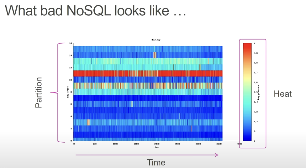
Another anti-pattern is Hot Keys. This means that most, if not all, access requests are hitting a single storage node, which means the key space has not been designed correctly.
The access heat map will look something like as follows:
DynamoDB
AWS DynamoDB is a fully managed, serverless, wide column key value store which means it supports many items, or rows, in a table but those items don’t necessarily have the same attributes. Data types that are supported are as follows:
- Scalar types: string, number, binary, boolean, null
- Document types: complex structure with nested attributes (i.e. JSON)
- Set types: string set, number set, binary set
As mentioned previously, NoSQL should be used when the application access patterns are well known, and there is a need to support a large number of TPS. DynamoDB can scale to any workload and will have a predictably fast and consistent response time of up to 4m TPS with low latency (10 - 20ms).
How does DynamoDB work?
Each item (or row) has a partition key that uniquely identifies that item and determines the data distribution across the underlying storage.
Items can optionally have a sort key, which determines the order in which the data is stored on disk within a partition. Sort keys allow us to query partitions with complex range and filter operations (although filter operations are applied at the client layer, not the database layer).
A partition key is used to create a hash index, and then each item is laid out according to this hash across a virtual key space. This virtual key space is divided into segments that map to physical storage devices, which can dynamically grow and shrink depending on the volume of data that is stored.
This is why DynamoDB is fast and consistent at any scale: because the database engine acts as a routing service from hashed keys to the physical storage.
Data Modeling with NoSQL
In this tutorial, we will model an online shop named Daintree.com.
(Fun fact: the Daintree rainforest, located in Queensland, Australia, is one of the oldest rainforests on Earth, estimated to be around 180 million years old!)
First, let’s create a highly oversimplified entity relationship diagram (ERD) so we can visualize what we are going to model.
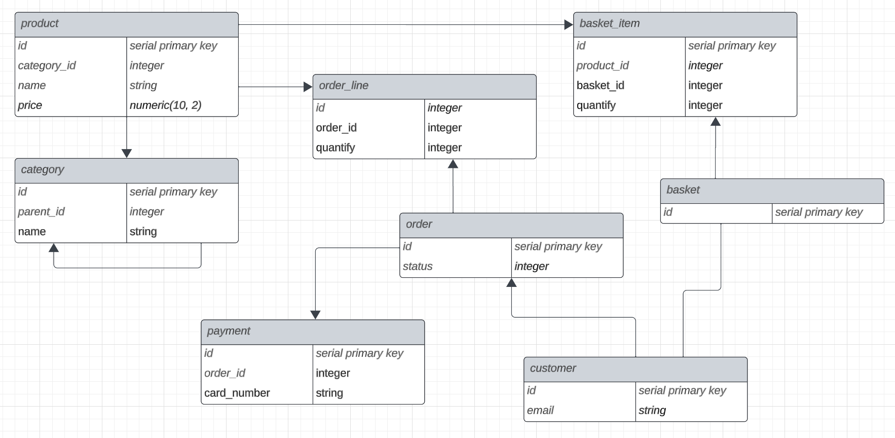
From this, we can deduce that a customer can create a shopping basket and add multiple products with varying quantities.
A product has a category, which in turn can have parent categories.
Baskets can become orders which can be split into multiple payments.
As already stated, this is a highly oversimplified view of the relationships and attributes of the entities that make up an online shopping application, but it serves the purpose of this tutorial.
Define the access patterns
We don’t need to worry about this step when implementing a relational database. SQL is an incredibly powerful language that, providing the schema has been designed correctly, allows us the flexibility to query and manipulate our data any way we see fit. This is not the case when using the single table design pattern in NoSQL because we need to store our data denormalized and ready for our application to directly consume.
Here are the access patterns we might want to support for our online shopping application:
- Query all products by category
- Query the subcategories for a parent category
- Query all orders by customer
- Query all payments for an order
- Query a specific order for a customer
- Query all basket items for a customer basket
- Query all products by customer order history
Modeling the table
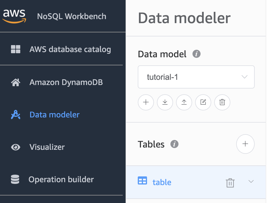
NoSQL workbench is a free tool provided by AWS to model NoSQL tables for DynamoDB.
Go to the Data modeler and create a new data model with a new table:
We are going to keep the primary key attributes as generic strings of PK and SK:
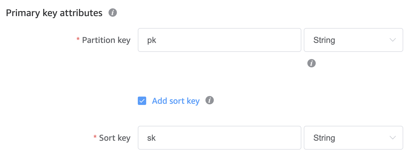
For additional attributes, we will store the entity_type along with two GSI PK and SK primary key attributes.
A GSI is a global secondary index, which is a copy of your table that DynamoDB keeps in sync (asynchronously!!) but stored using alternative primary key attribute pairs. This is the key mechanism for how a single table can support multiple access patterns. More on this topic later; for now, just understand that these keys will store the primary keys of related entities.
The other additional attributes we need to add are all the non-key attributes of our data (note this step is only required for the design phase and won’t be explicitly defined when we provision the actual table):
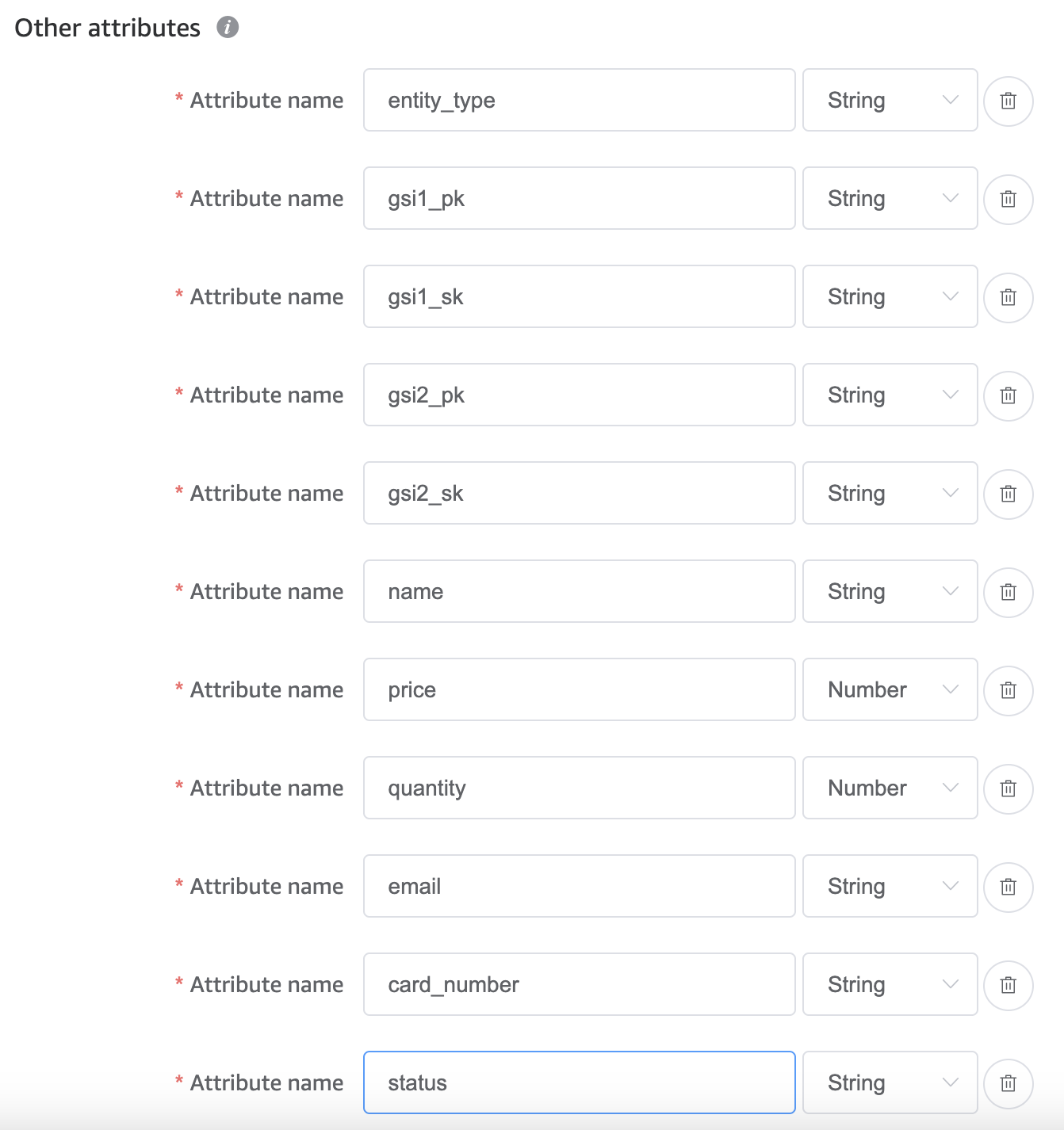
Next, we add the two GSI’s using the keys we defined in the previous step:
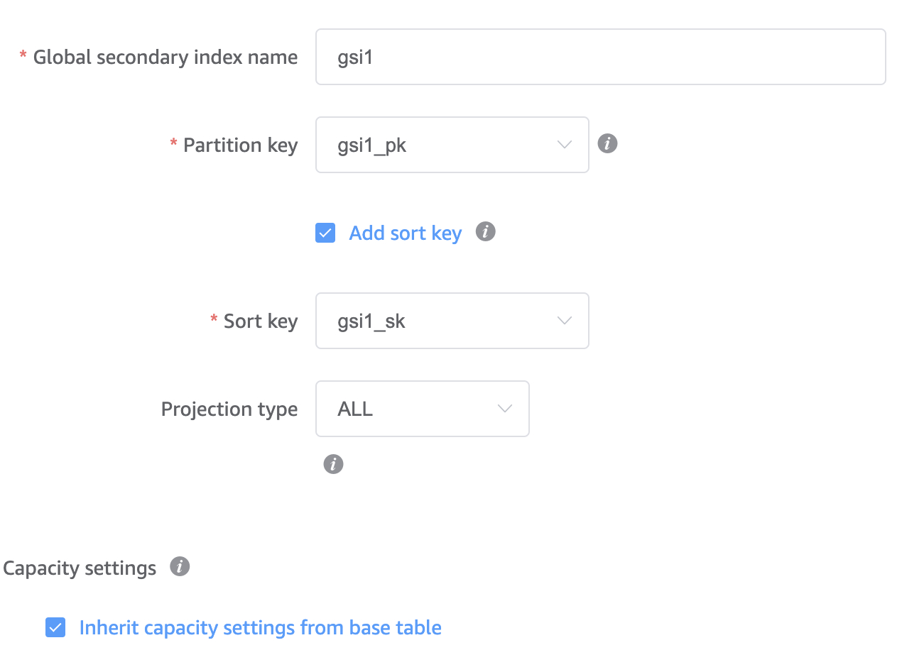
Hit save and then click to visualize the data model. You should now see your newly created but empty table. Click edit table, then in the top right, edit data; this will allow you to add new rows:

Data prefixes
Before we start adding data, we need to define our primary key prefixes for each entity:
|
product |
p# |
|
category |
c# |
|
customer (user) |
u# |
|
basket |
b# |
|
basket item |
bi# |
|
order |
o# |
|
order line |
ol# |
|
payment |
py# |
|
invoice |
i# |
Modeling the data
Customer data
The majority of access patterns revolve around the customer, so for our primary index, we will use the customer ID as the main partition, with the actual customer record being identifiable with the sort key also being the customer ID.
We can then easily add relationships of customers to orders and customers to baskets by using the same partition key but with a unique sort key.
Our aggregate view now looks like this:
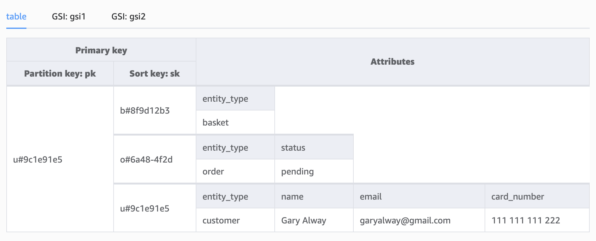
We can now query all three records in a single command, querying that entire customers’ partition:
export const getAllCustomerRecords = async (id: string) =>
  dynamoClient
    .query({
      TableName: TABLE_NAME,
      KeyConditionExpression: "pk=:pk",
      ExpressionAttributeValues: {
        ":pk": valueToAttributeValue(addPrefix(id, CUSTOMER_PREFIX)),
      },
    })
    .then((result) => result.Items);
As the table grows, this sort of query might not be the most efficient given it will return every customer order ever made, along with all the other customer records such as baskets and invoices, but it's good to know we can access all customer data in a single query should we need to.
A small tweak to the expression attribute values to include a partial match (begins_with) on the sort key allows us to query:
- All customer basket records
- All customer order records
The important takeaway is how we can model one-to-one and one-to-many relationships in NoSQL.
Categories
These entities represent another one-to-many relationship where one category can contain many products.
Categories also have a hierarchical relationship where a category can have many subcategories, meaning products can exist anywhere in the category hierarchy tree.
Let’s model this with books broken down into fiction and non-fiction.
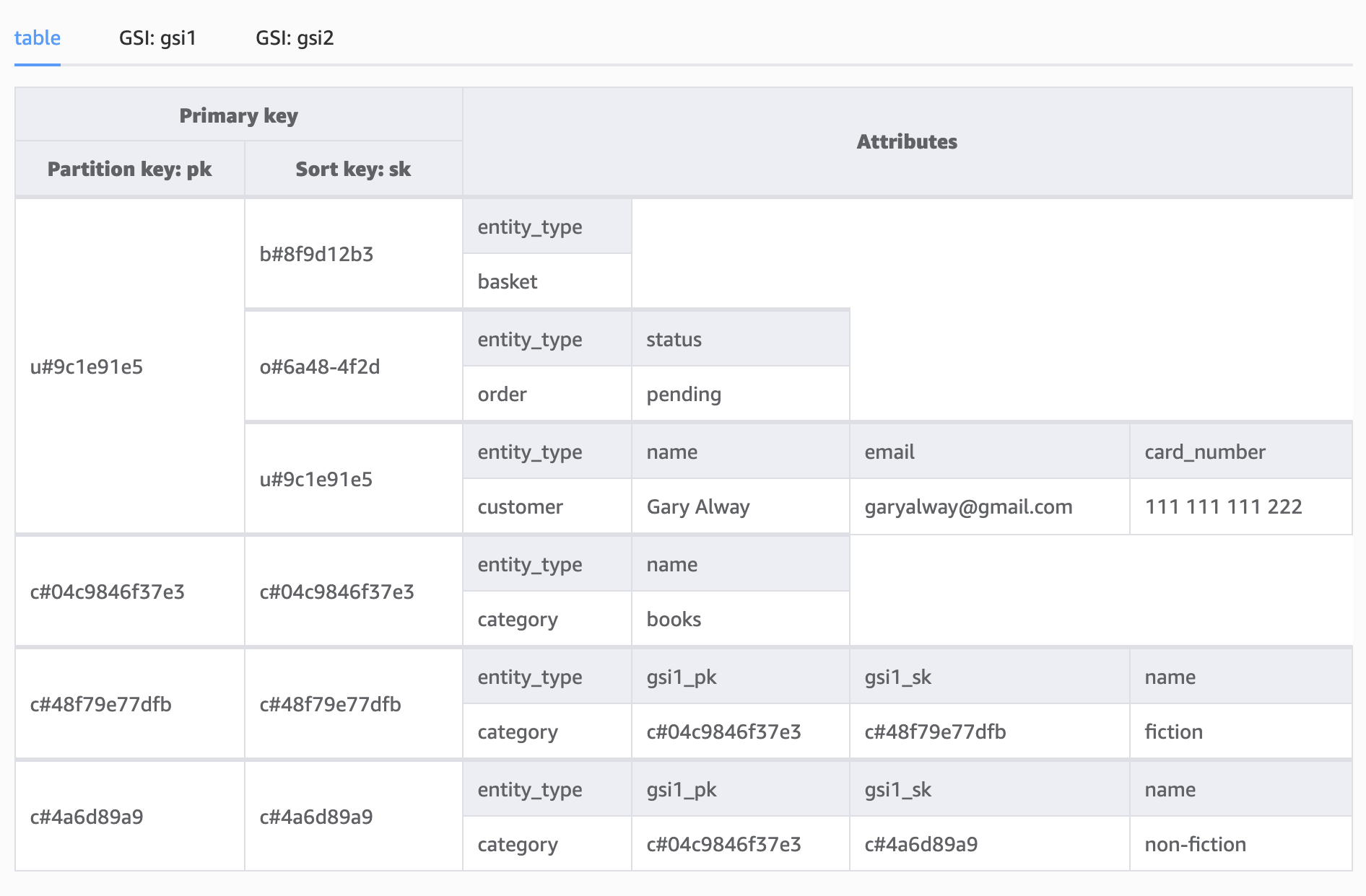
Notice how we have populated the GSI attribute keys for the subcategories, setting the GSI1_PK as the parent category ID and the GSI1_SK as the subcategory ID. This allows us to query all of the subcategories by category using GSI1:

The same index, GSI1, can be used not only for mapping one to many relationships. Say for example we want to look up the customer by email,; thecurrent model doesn’t support this directly unless we make a slight change in the way we save the data:
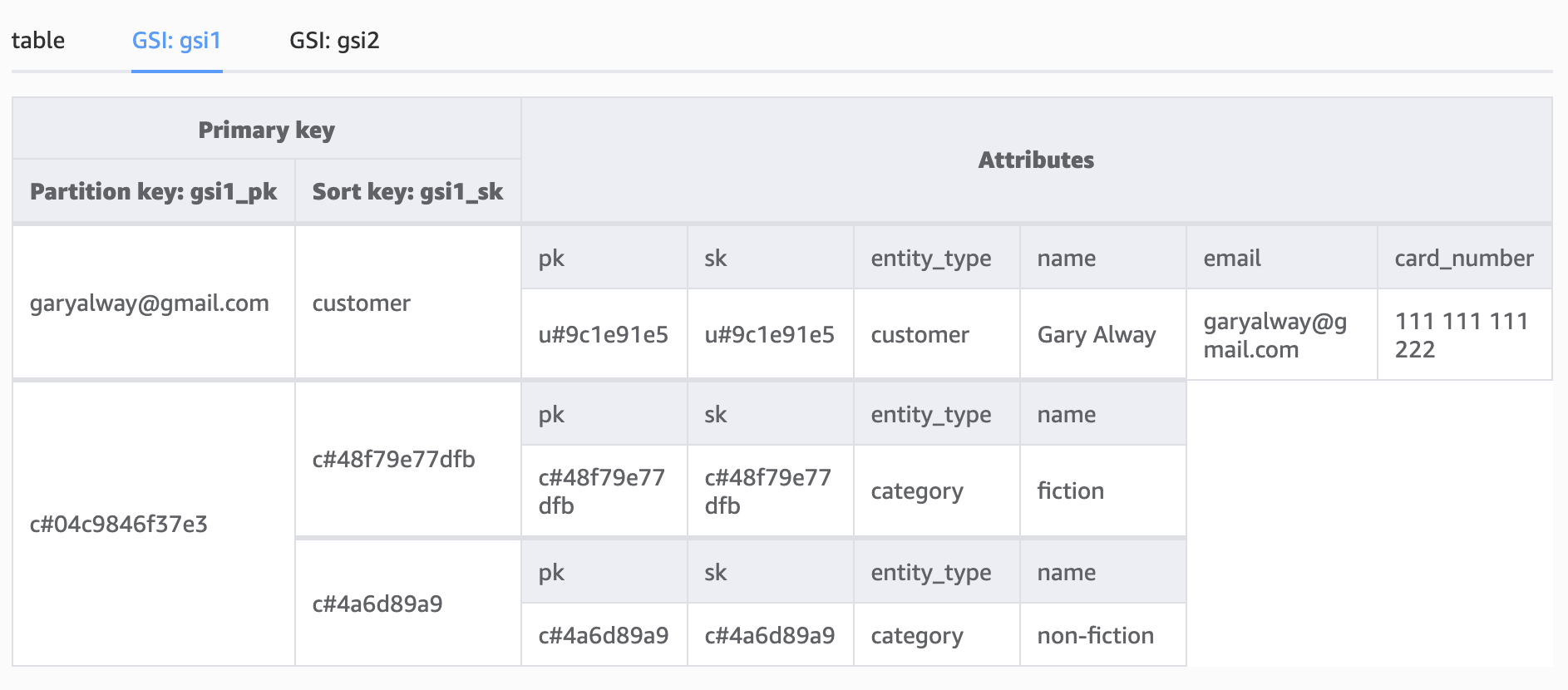
Storing the customer email address and entity type as GSI PK and SK;
- Ensures the customer email address is unique (for this GSI only, enforcing uniqueness on the primary index would need to have another solution)
- Allows for customers to also appear as sellers, for example (if we had that as an entity type)
- Allows us to look up a customer by email rather than by ID
To assist in DynamoDB data distribution, we could take this a step further by storing the email address as a hash.
export const getCustomerByEmail = async (email: string) =>
  dynamoClient
    .query({
      TableName: TABLE_NAME,
      IndexName: "gsi1",
      KeyConditionExpression: "gsi1_pk = :email AND gsi1_sk = :entityType",
      ExpressionAttributeValues: {
        ":email": valueToAttributeValue(email),
        ":entityType": valueToAttributeValue(entityType),
      },
    })
    .then(({ Items }) => Items?.[0]);
Up until now, you may have wondered why all the indexes had generic names with generically named key attributes of just PK and SK. The answer should now be clear: the data we store and the indexes we maintain are flexible and capable of supporting multiple access patterns depending on the entity type.
The terraform for the table we have been using so far is as follows:
resource "aws_dynamodb_table" "tutorial-1" {
  name = "tutorial-1"
  billing_mode = "PAY_PER_REQUEST"
  hash_key = "pk"
  range_key = "sk"


  attribute {
    name = "pk"
    type = "S"
  }


  attribute {
    name = "sk"
    type = "S"
  }


  attribute {
    name = "gsi1_pk"
    type = "S"
  }


  attribute {
    name = "gsi1_sk"
    type = "S"
  }


  attribute {
    name = "gsi2_pk"
    type = "S"
  }


  attribute {
    name = "gsi2_sk"
    type = "S"
  }


  global_secondary_index {
    name = "gsi1"
    hash_key = "gsi1_pk"
    range_key = "gsi1_sk"
    projection_type = "ALL"
  }


  global_secondary_index {
    name = "gsi2"
    hash_key = "gsi2_pk"
    range_key = "gsi2_sk"
    projection_type = "ALL"
  }
}
Products
Storing products follows the same one to many pattern where the partition key is the category ID and the sort key is the product ID:

Adding the parent category to GSI1 allows us to query all the books in our database:

In a production application, we can use DynamoDB streams to push data to an Elasticsearch cluster giving us the ability to search by book title, but how could we use our existing model to query by product title?
We have already used GSI1, so we could use GSI2 for this:
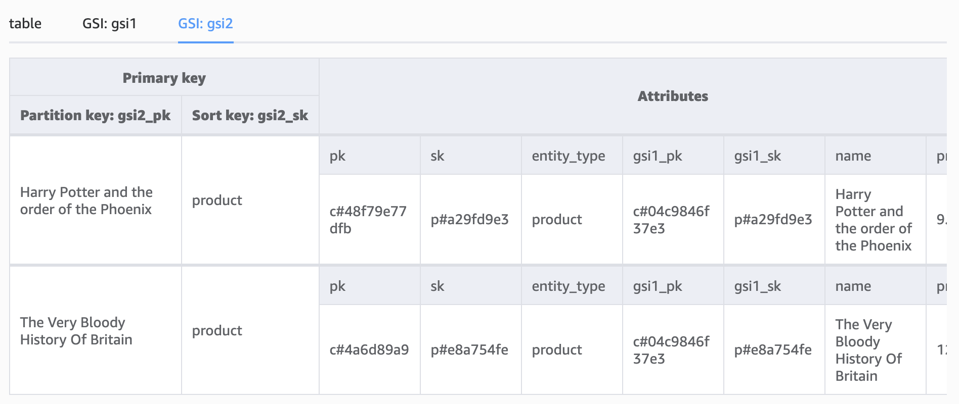
Remember, when querying DynamoDB, you need to provide the full exact partition key, so while this implementation may not be the most optimal, it does illustrate how three indexes can be used for different access patterns.
In my next tutorial, I will demonstrate how this can be solved by integrating it with a search index.
Basket contents and order lines
Both basket items and order lines are stored in the customer partition; we can use the GSIs to allow us to query all the products in a basket, all the products in an order, and all of the products a customer has ever ordered.
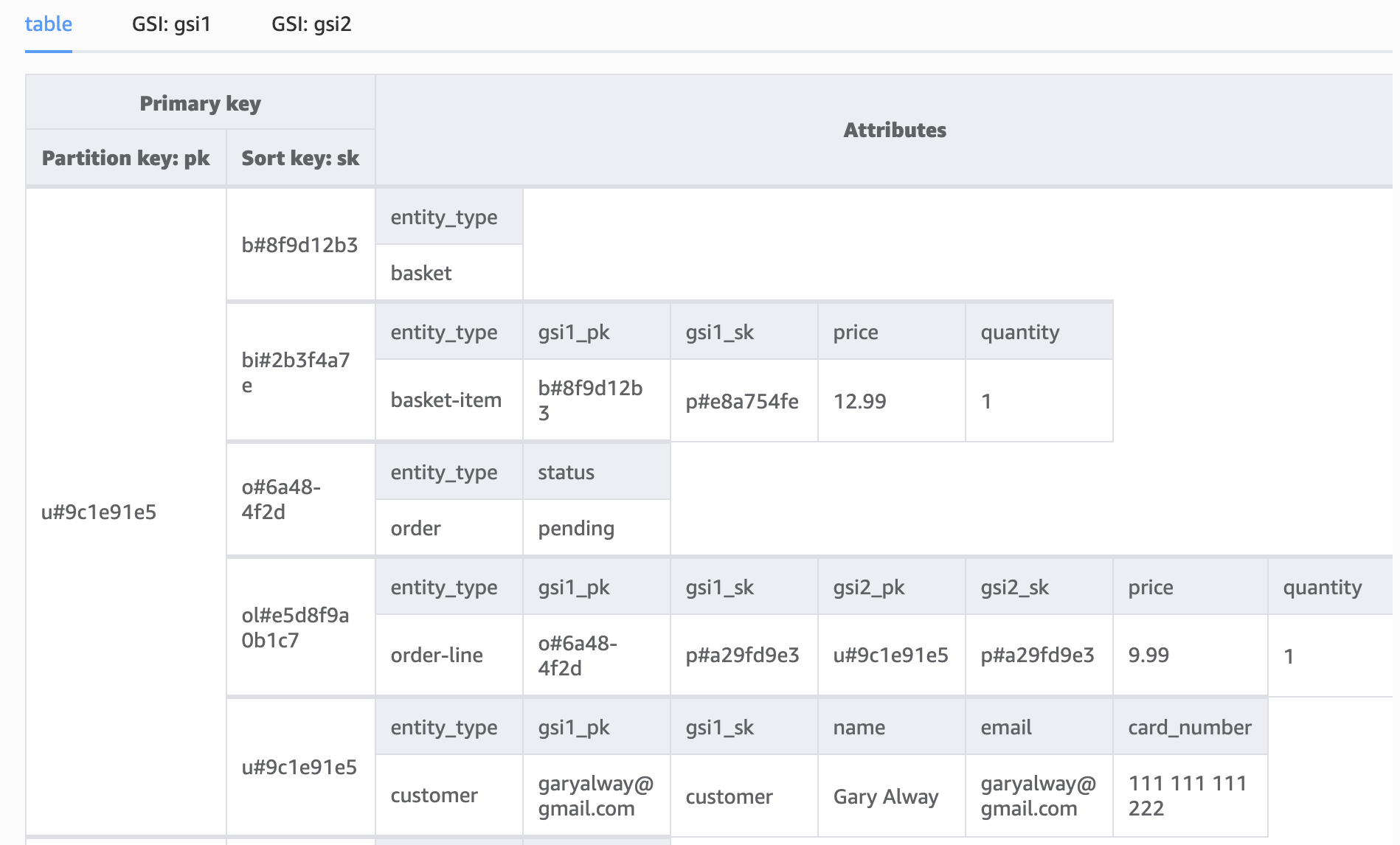
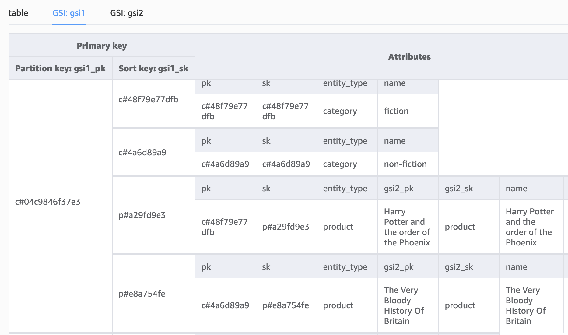
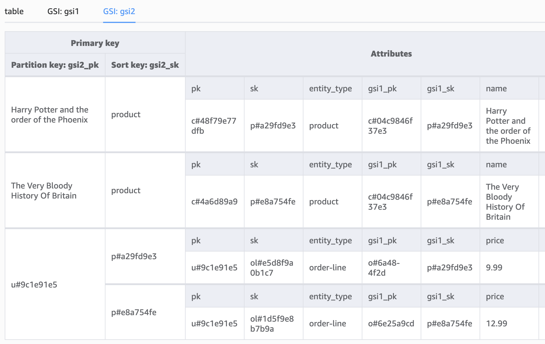
This final example shows a customer’s order history with two products made from two different order IDs.
For those interested in how data modeling works in SQL databases, our Data Modeling in SQL webinar offers valuable insights that can complement your understanding of NoSQL data modeling.
Challenges Associated with Single Table Design
Using a single table design with DynamoDB offers many advantages, but it also presents several challenges and considerations:
Complexity and application logic
Managing all your data in a single table can become complex, especially as your application grows and evolves.
You must carefully plan and structure your data to accommodate various query patterns. Additionally, the effectiveness of a single table design is closely tied to your application logic; it plays a pivotal role in ensuring smooth data access and efficient query processing.
Careful consideration of both data structure and application logic is essential for a single table design to work effectively.
Index overhead
While DynamoDB allows for Global Secondary Indexes to support different query patterns, you need to provision and maintain these indexes, which can increase costs and complexity.
Partition key selection
Choosing the right partition key is critical for even data distribution and query performance. Picking an unsuitable partition key can lead to hot partitions and performance bottlenecks.
Size and cost
As your data volume increases, your single table can grow significantly in size. This can affect both the cost of storage and the cost of reading and writing data.
No full-text search
DynamoDB doesn't natively support full-text search, so implementing such functionality requires integrating with other services like Elasticsearch.
Schema changes
Making changes to your table schema can be challenging, especially in production systems. You might need to migrate existing data or modify your application logic to accommodate schema changes.
Consistency considerations
Depending on your choice of read consistency (strong or eventual), you may need to account for potential data consistency challenges, keeping in mind that GSIs are replicated asynchronously.
Limited query flexibility
DynamoDB's query capabilities are powerful but not as flexible as SQL queries.
To better understand how to design databases effectively and navigate associated challenges, check out our Database Design course.
Conclusion
When working with a NoSQL database, it's crucial to break away from the familiar territory of relational database design patterns; you must unlearn what you have learned.
Opting for the single table design pattern offers the promise of a globally scalable database ready to handle large volumes of traffic with dependable and predictable performance.
However, this performance advantage doesn't come free; it demands meticulous planning and thoughtful implementation of your database structure and application logic upfront.
Follow up on your knowledge with our NoSQL concepts course!

I'm a Full stack Software Engineer and Solutions Architect with a passion for learning and data!


