
课程
Python 中的 LLM 入门
3 小时
36.6K
Google 刚刚发布了 Gemma 4,称其为迄今为止最智能的开源模型家族,面向强推理与智能体工作流而构建。Gemma 模型在不同环境中均具备良好的灵活性,官方支持本地开发、云端部署和模型定制的工具链,非常适合进行微调项目。
在本教程中,我们将对 Gemma 4 E4B-it 执行微调,所用数据集来自 Hugging Face 的人类情绪分类数据集。我们将搭建 3090 GPU 环境,加载并检查数据集,准备与格式化用于监督微调的数据,加载基础模型、在训练前进行基线评估、微调模型,并在训练后再次评估其表现。
首先启动一个新的 Runpod 实例,并确保您的账户在开始前至少有 $5 余额。本教程请选择一个 3090 GPU pod,并选用最新的 PyTorch 模板。
部署前,打开模板设置并进行一些调整。将 container disk 和 volume disk 均增加到 40 GB,以便有足够空间存放模型、数据集、缓存文件和训练检查点。
您还应将 Hugging Face 令牌添加为环境变量。您可以在 Hugging Face 账户的 Settings > Access Tokens 中生成该令牌。
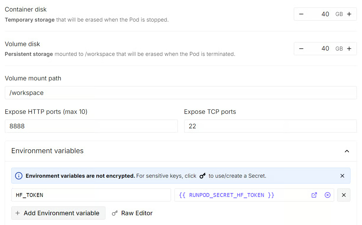
设置完成后,部署该 pod。实例启动可能需要一两分钟。就绪后,打开 JupyterLab 界面,开始在该环境中工作。
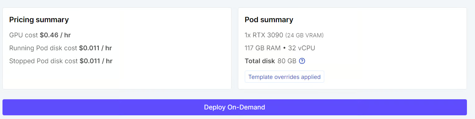
进入 JupyterLab 后的第一步,是新建一个 Python 笔记本并安装所有必需的 Python 包。在笔记本单元中运行以下命令:
%%capture
!pip install -U transformers accelerate datasets trl peft bitsandbytes scikit-learn huggingface_hub
这些包覆盖完整流程,包括加载数据集、准备模型、微调与评估。
最后一步是使用已保存的令牌登录 Hugging Face Hub。这样您即可访问受限模型,并更方便地上传文件、创建仓库以及后续推送微调后的模型。
import os
from huggingface_hub import login

hf_token = os.environ.get("HF_TOKEN")
if not hf_token:
    raise ValueError("Set HF_TOKEN in the RunPod environment before running this notebook.")

login(token=hf_token)
print("Logged in to Hugging Face.")环境就绪后,下一步从 Hugging Face 加载情绪数据集,并为训练与评估准备更小的切分集。
在本教程中,我们不使用完整数据集,而是创建受限的训练、验证和测试切分,以便微调过程更快、在单块 GPU 上更易运行。
from datasets import load_dataset, DatasetDict

TRAIN_LIMIT = 4000
VALIDATION_LIMIT = 400
TEST_LIMIT = 400
EVAL_LIMIT = 400

raw_dataset = load_dataset("dair-ai/emotion")

def maybe_limit(split, limit):
    split = split.shuffle(seed=42)
    if limit is None:
        return split
    return split.select(range(min(limit, len(split))))

dataset = DatasetDict({
    "train": maybe_limit(raw_dataset["train"], TRAIN_LIMIT),
    "validation": maybe_limit(raw_dataset["validation"], VALIDATION_LIMIT),
    "test": maybe_limit(raw_dataset["test"], TEST_LIMIT),
})

dataset
最终数据集包含 4,000 个训练样本、400 个验证样本和 400 个测试样本。
DatasetDict({
    train: Dataset({
        features: ['text', 'label'],
        num_rows: 4000
    })
    validation: Dataset({
        features: ['text', 'label'],
        num_rows: 400
    })
    test: Dataset({
        features: ['text', 'label'],
        num_rows: 400
    })
})
接着查看数据集中存储的标签名称。模型将学习预测这些情绪类别。
label_names = dataset["train"].features["label"].names
label_names
这表明任务包含六类情绪:sadness、joy、love、anger、fear 和 surprise。
['sadness', 'joy', 'love', 'anger', 'fear', 'surprise']我们还可以检查训练切分中的一个样本,了解数据结构。
dataset["train"][0]每个样本包含一段文本和一个数值标签。在此示例中,标签 4 对应上述标签列表中的 fear。
{'text': 'while cycling in the country', 'label': 4}在微调模型之前,我们需要将数据集转换为 Gemma 4 训练时所用的格式。
我们不直接传入原始文本和标签,而是将每个样本组织为一段简短的对话:包含 system 消息、user 消息以及预期的 assistant 回复。
system 提示明确告诉模型需要执行的任务。本例中,我们希望模型充当情绪分类助手,并只返回六个允许标签中的一个。
SYSTEM_PROMPT = """You are an emotion classification assistant.
Read the user's text and answer with exactly one label.
Only choose from: sadness, joy, love, anger, fear, surprise.
Return only the label and nothing else."""在该设置下,user 消息包含待分类的输入文本,而assistant 消息包含正确标签。这是用于监督微调的格式,模型将学习为每个训练样本生成正确回复。
def to_prompt_completion(example):
    text = example["text"]
    label = label_names[example["label"]]
    return {
        "prompt": [
            {
                "role": "system",
                "content": SYSTEM_PROMPT,
            },
            {
                "role": "user",
                "content": f"Classify the emotion of this text:\n\n{text}",
            },
        ],
        "completion": [
            {
                "role": "assistant",
                "content": label,
            }
        ],
    }

sft_dataset = dataset.map(to_prompt_completion, remove_columns=dataset["train"].column_names)
应用此格式化函数后,原始的 text 和 label 列被结构化的 prompt 和 completion 字段替代。
我们可以检查一个样本,确认数据集已正确格式化。
sft_dataset["train"][0]输出清晰展示了完整训练结构。模型看到指令,读取输入文本,并学习将正确的情绪标签作为答案生成。
{'prompt': [{'content': "You are an emotion classification assistant.\nRead the user's text and answer with exactly one label.\nOnly choose from: sadness, joy, love, anger, fear, surprise.\nReturn only the label and nothing else.",
   'role': 'system'},
  {'content': 'Classify the emotion of this text:\n\nwhile cycling in the country',
   'role': 'user'}],
'completion': [{'content': 'fear', 'role': 'assistant'}]}现在可以加载 Gemma 4 E4B-it 并为微调做好准备。鉴于该模型相对较大,我们使用 4 比特量化以降低内存占用,使其更易在 3090 GPU 上运行。我们还将计算类型设为 bfloat16,以提升效率。
先导入所需库并定义主要模型设置。
import torch
from transformers import AutoModelForCausalLM, AutoTokenizer, BitsAndBytesConfig

MODEL_ID = "google/gemma-4-E4B-it"
MODEL_DTYPE = torch.bfloat16
USE_4BIT = True
接着启用部分 CUDA 优化并加载分词器。
if torch.cuda.is_available():
    torch.backends.cuda.matmul.allow_tf32 = True
    torch.backends.cudnn.allow_tf32 = True

processor = AutoTokenizer.from_pretrained(MODEL_ID, use_fast=True)
if processor.pad_token is None:
    processor.pad_token = processor.eos_token
现在准备量化设置与模型加载参数。
bnb_config = None
model_kwargs = {
    "device_map": "auto",
}
if USE_4BIT:
    bnb_config = BitsAndBytesConfig(
        load_in_4bit=True,
        bnb_4bit_quant_type="nf4",
        bnb_4bit_compute_dtype=MODEL_DTYPE,
    )
    model_kwargs["quantization_config"] = bnb_config
else:
    model_kwargs["torch_dtype"] = MODEL_DTYPE
最后加载模型,并将其配置与分词器对齐。
base_model = AutoModelForCausalLM.from_pretrained(MODEL_ID, **model_kwargs)
base_model.config.use_cache = False
base_model.config.pad_token_id = processor.pad_token_id
base_model.config.bos_token_id = processor.bos_token_id
base_model.config.eos_token_id = processor.eos_token_id
base_model.generation_config.pad_token_id = processor.pad_token_id
base_model.generation_config.bos_token_id = processor.bos_token_id
base_model.generation_config.eos_token_id = processor.eos_token_id

print(f"Base model loaded with 4-bit={USE_4BIT} and dtype={MODEL_DTYPE}.")
这会将基础模型加载到可用设备上,关闭训练时缓存,并确保特殊 token ID 在模型配置与生成配置中均设置正确。
Base model loaded with 4-bit=True and dtype=torch.bfloat16.在微调之前,先评估基础模型以获取清晰的对照基线非常有用。
本节定义若干辅助函数,用于生成预测、提取有效情绪标签,并在测试切分上进行评估。
首先创建一个简单的标签提取模式和预测辅助函数。
这些函数涵盖完整预测流程。模型以对话格式接收输入,生成简短回复,然后我们提取预测标签。若模型返回了额外文本,辅助函数会尝试恢复首个有效情绪标签。
import re

LABEL_PATTERN = re.compile(r"\b(sadness|joy|love|anger|fear|surprise)\b", re.IGNORECASE)

def extract_label(raw_text: str) -> str:
    raw_text = raw_text.strip().lower()
    match = LABEL_PATTERN.search(raw_text)
    if match:
        return match.group(1)

    first_token = raw_text.split()[0].strip(".,!?:;\"'()[]{}") if raw_text.split() else ""
    return first_token

def generate_label(model, processor, user_text, system_prompt, max_new_tokens=4):
    messages = [
        {
            "role": "system",
            "content": system_prompt,
        },
        {
            "role": "user",
            "content": f"Classify the emotion of this text:\n\n{user_text}",
        },
    ]

    device = next(model.parameters()).device
    inputs = processor.apply_chat_template(
        messages,
        tokenize=True,
        add_generation_prompt=True,
        return_dict=True,
        return_tensors="pt",
    ).to(device)

    input_len = inputs["input_ids"].shape[-1]

    with torch.no_grad():
        outputs = model.generate(
            **inputs,
            max_new_tokens=max_new_tokens,
            do_sample=False,
            pad_token_id=processor.pad_token_id,
            eos_token_id=processor.eos_token_id,
        )

    raw_pred = processor.decode(outputs[0][input_len:], skip_special_tokens=True).strip()
    return extract_label(raw_pred)


def predict_emotion(user_text: str, model=None, proc=None) -> str:
    model = model or base_model
    proc = proc or processor
    return generate_label(model, proc, user_text, SYSTEM_PROMPT)
现在我们可以在单个样本上测试设置,然后再运行完整评估。
predict_emotion("I feel so happy and excited today!")该样例预测看起来正确,接下来即可在测试切分上评估模型。
'joy'以下代码在测试切分上评估模型并收集多项有用输出。它存储真实与预测标签,记录每个预测是否正确,并返回汇总指标、分类报告以及包含全部预测的数据框。
from sklearn.metrics import accuracy_score, classification_report, confusion_matrix, f1_score
import pandas as pd
from tqdm.auto import tqdm

VALID_LABELS = set(label_names)
ALL_EVAL_LABELS = label_names + ["INVALID"]

def evaluate_model(model, processor, split="test", limit=EVAL_LIMIT):
    y_true, y_pred, rows = [], [], []
    raw_source = dataset[split]
    if limit is not None:
        raw_source = raw_source.select(range(min(limit, len(raw_source))))

    model.eval()

    for ex in tqdm(raw_source, desc=f"Evaluating {split}", leave=False):
        true_label = label_names[ex["label"]]
        raw_pred_label = generate_label(model, processor, ex["text"], SYSTEM_PROMPT)
        pred_label = raw_pred_label if raw_pred_label in VALID_LABELS else "INVALID"

        y_true.append(true_label)
        y_pred.append(pred_label)
        rows.append({
            "text": ex["text"],
            "true_label": true_label,
            "pred_label": pred_label,
            "raw_pred_label": raw_pred_label,
            "correct": true_label == pred_label,
        })

    metrics = {
        "accuracy": accuracy_score(y_true, y_pred),
        "macro_f1": f1_score(y_true, y_pred, labels=label_names, average="macro", zero_division=0),
        "invalid_predictions": sum(1 for p in y_pred if p == "INVALID"),
        "evaluated_examples": len(y_true),
    }

    report = classification_report(
        y_true,
        y_pred,
        labels=label_names,
        output_dict=True,
        zero_division=0,
    )

    df = pd.DataFrame(rows)
    return metrics, report, df

def confusion_matrix_df(pred_df):
    return pd.DataFrame(
        confusion_matrix(pred_df["true_label"], pred_df["pred_label"], labels=ALL_EVAL_LABELS),
        index=ALL_EVAL_LABELS,
        columns=ALL_EVAL_LABELS,
    )
现在可以在基础模型上运行完整的基线评估。
pre_metrics, pre_report, pre_preds = evaluate_model(base_model, processor, "test")
pre_metrics
这些基线结果显示,未微调模型已经有一定表现,但仍有提升空间。
准确率约为 58.25%,宏平均 F1 约为 0.42,且模型产生了 33 次无效预测,意味着它有时返回了不在期望标签集内的内容。
{'accuracy': 0.5825,
 'macro_f1': 0.42112912841373906,
 'invalid_predictions': 33,
 'evaluated_examples': 400}
接下来查看各情绪类别的完整分类报告。
pd.DataFrame(pre_report).transpose()这将给出每一类的精确率、召回率、F1 分数与支持度。它有助于在微调前了解模型擅长与薄弱的情绪类别。
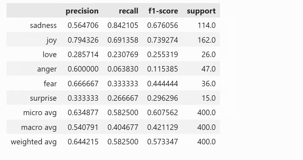
最后,我们查看混淆矩阵。
confusion_matrix_df(pre_preds)混淆矩阵展示了预测在不同类别间的分布情况。
在笔记本中,它会以表格形式显示,便于发现哪些情绪彼此混淆,以及基础模型最容易出错的地方。
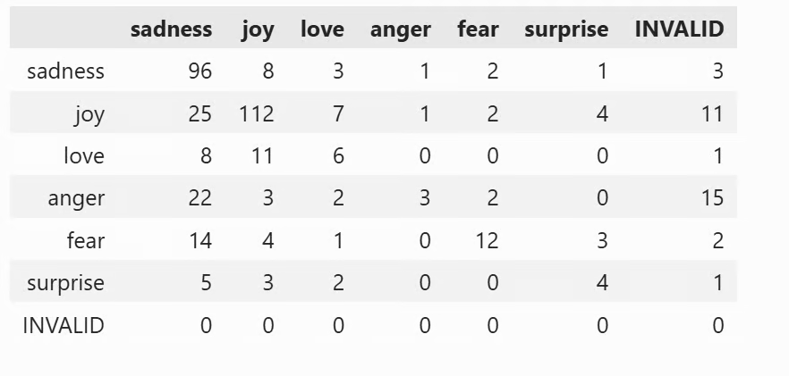
有了基线结果后,我们使用 LoRA 对 Gemma 4 进行微调。
LoRA 是一种参数高效的微调方法,意味着我们不会更新整个模型,而是在基础模型之上挂载少量可训练的适配器权重。这样训练更轻量,也更适合单块 GPU 实践。
我们先定义 LoRA 配置。
这些设置控制 LoRA 适配器如何挂载到模型。这里使用秩 16、dropout 0.05,并将 LoRA 应用于所有线性层,这是高效微调的常见配置。
from peft import LoraConfig

lora_config = LoraConfig(
    r=16,
    lora_alpha=32,
    lora_dropout=0.05,
    bias="none",
    task_type="CAUSAL_LM",
    target_modules="all-linear"
)
接下来定义训练配置并设置训练器。
该训练设置旨在控制内存占用,同时为模型提供足够的学习空间。我们训练 1 个 epoch,使用梯度累积来模拟更大的批量,并启用如梯度检查点与 8 比特优化等选项以提升训练效率。
from trl import SFTConfig, SFTTrainer

training_args = SFTConfig(
    output_dir="./gemma4-emotion-lora",
    per_device_train_batch_size=8,
    per_device_eval_batch_size=8,
    gradient_accumulation_steps=2,
    learning_rate=1e-4,
    weight_decay=0.01,
    lr_scheduler_type="linear",
    warmup_steps=50,
    num_train_epochs=1,
    logging_steps=50,
    eval_strategy="steps",
    metric_for_best_model="eval_loss",
    greater_is_better=False,
    gradient_checkpointing=True,
    bf16=True,
    fp16=False,
    tf32=True,
    max_length=256,
    packing=False,
    completion_only_loss=True,
    remove_unused_columns=False,
    dataloader_num_workers=2,
    optim="paged_adamw_8bit",
    report_to="none",
)
现在确认基础模型就绪并初始化训练器。该步骤将 LoRA 适配器挂载到基础模型上,并使用我们格式化的训练与验证切分来准备监督微调训练器。
from peft import PeftModel

if isinstance(base_model, PeftModel):
    base_model = base_model.unload()
    base_model.config.use_cache = False

trainer = SFTTrainer(
    model=base_model,
    train_dataset=sft_dataset["train"],
    eval_dataset=sft_dataset["validation"],
    peft_config=lora_config,
    args=training_args,
    processing_class=processor,
)
开始训练前,最好确认 LoRA 参数已正确挂载。
以下代码统计可训练参数数量,若未添加任何 LoRA 层则抛出错误。
之后开始训练。
trainable_params = 0
for param in trainer.model.parameters():
    if param.requires_grad:
        trainable_params += param.numel()

if trainable_params == 0:
    raise RuntimeError("No trainable LoRA parameters were attached. Check target_modules before training.")

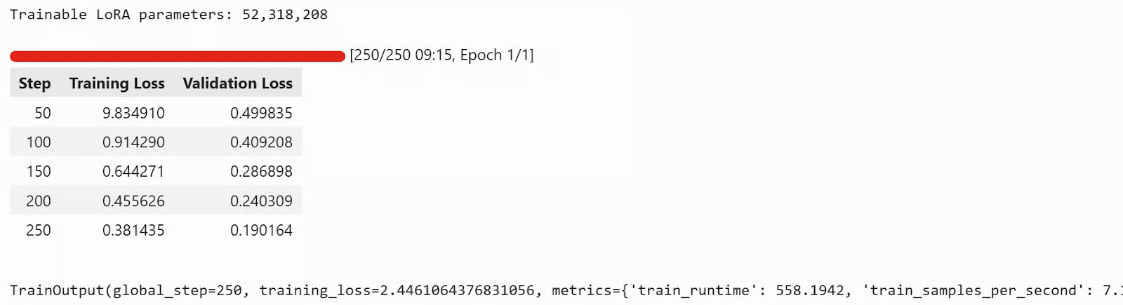
print(f"Trainable LoRA parameters: {trainable_params:,}")
train_result = trainer.train()
trainer.model.eval()
trainer.model.config.use_cache = True
train_result
本次运行中,训练耗时接近 9 分钟,训练损失与验证损失均持续下降,表明模型从数据集中确实学到了模式。
训练完成后,我们可将适配器与分词器保存在本地。
trainer.model.save_pretrained("./gemma4-emotion-lora")
processor.save_pretrained("./gemma4-emotion-lora")
最后,我们可以将模型推送到 Hugging Face Hub。
这会将微调后的适配器与分词器上传至 Hub,方便您随处访问、与他人分享,或直接在其他笔记本或应用中加载。
repo_id = "kingabzpro/gemma4-emotion-lora"

# Push adapter + processor to the Hub
trainer.model.push_to_hub(
    repo_id,
    private=False,
)

processor.push_to_hub(
    repo_id,
    private=False,
)
您现在可以在 Hugging Face 查看 kingabzpro/gemma4-emotion-lora 并亲自试用。该仓库包含模型文件、使用说明及微调结果。
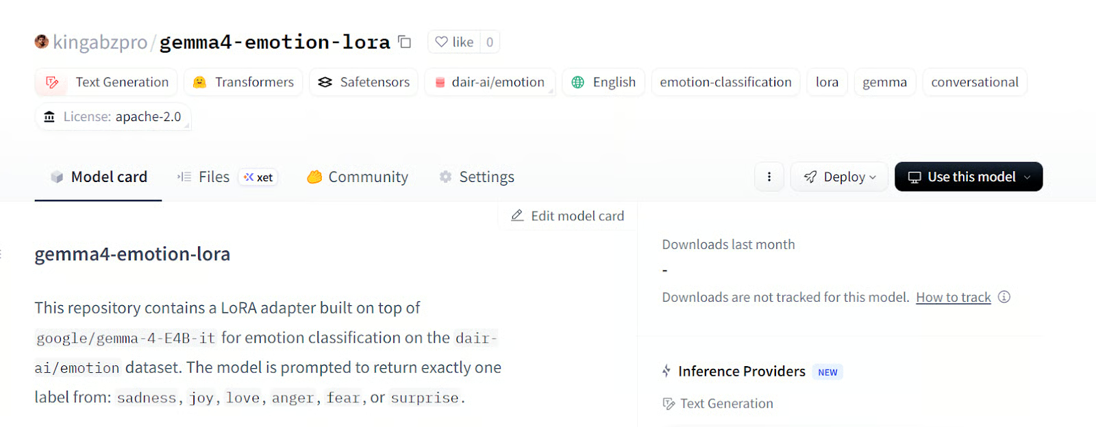
来源: kingabzpro/gemma4-emotion-lora · Hugging Face
训练完成后,最后一步是在同一测试切分上评估微调后的模型,并与基础模型对比。这能帮助我们判断 LoRA 微调是否提升了模型的情绪分类准确性。
我们先从训练器中加载微调模型并运行评估。
ft_model = trainer.model
ft_model.eval()
ft_model.config.use_cache = True
post_metrics, post_report, post_preds = evaluate_model(ft_model, processor, "test")
post_metrics
这给出了微调模型的主要评估指标。
这些结果明显强于基线。微调后,模型达到 77.25% 的准确率与 0.698 的宏平均 F1。无效预测数量也从 33 降至 20,说明微调后的模型不仅更准确,也更稳定地返回有效标签。
{'accuracy': 0.7725,
 'macro_f1': 0.697702361480462,
 'invalid_predictions': 20,
 'evaluated_examples': 400}
接下来查看完整分类报告。
它会在笔记本中以 pandas DataFrame 的形式显示分类报告,包含每个情绪类别的 精确率、召回率、F1 分数与支持度,便于观察微调后提升最大的类别。
pd.DataFrame(post_report).transpose()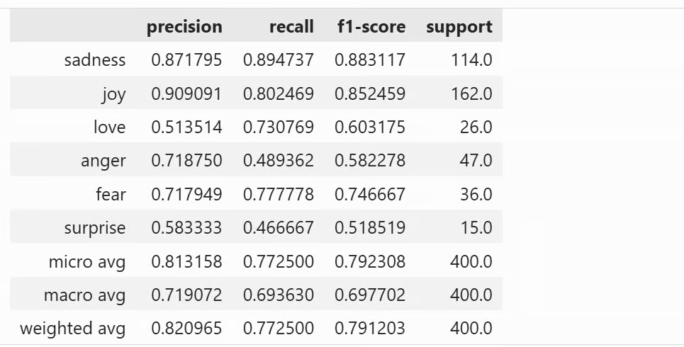
这也会在笔记本中以表格显示。它帮助您了解微调后模型仍在哪些方面出错、哪些情绪类别最易互相混淆。
confusion_matrix_df(post_preds)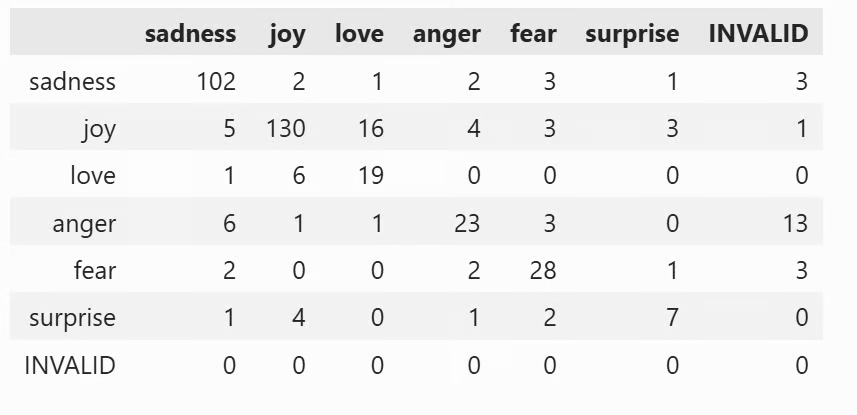
为便于对比,我们将微调前与微调后的指标并排展示。
comparison_df = pd.DataFrame([
    {"stage": "pre_finetuning", **pre_metrics},
    {"stage": "post_finetuning", **post_metrics},
])
comparison_df
它可快速概览训练后模型的提升幅度。

注意: 如果您在运行代码时遇到任何问题,可参考完整的 Jupyter 笔记本: fine-tune-gemma-4-on-emotions_final.ipynb
微调 Gemma 4 对设置十分敏感,尤其是 提示词结构与训练参数。如果提示词格式不正确,或未始终如一地使用合适模板,模型可能经历训练却并未真正学会任务。训练设置亦然。这些通常是损失不下降,或损失下降但评估结果改进甚微的主要原因。
另一个重要经验是 max_length。如果将其压得过低,尤其低于约 125,模型可能根本无法学到正确模式。在此过程中我也遇到过若干问题,但它们都被逐一解决了,而大多回到了同两点:提示词格式与训练配置。
如需进一步提升结果,下一步可在 完整数据集上微调,并将训练轮数从 1 提高到至少 3 个 epoch。这将为模型提供更多学习样本与适应时间,通常能带来更高的准确率与 F1 分数。
与 DataCamp 一起学习
课程
课程
课程