A Comprehensive Introduction to Anomaly Detection

Semua orang senang jadi perhatian, tampil beda. Namun, itu bukanlah sifat yang Anda inginkan dari titik data saat menjadi data scientist. Titik data yang menyimpang, atau anomali, dalam sebuah dataset adalah salah satu masalah kualitas data paling berbahaya yang menghantui hampir semua proyek data.

Kalimat terakhir ini mungkin mengejutkan jika Anda hanya bekerja dengan dataset open-source yang rapi dan sering kali tanpa pencilan. Namun, dataset dunia nyata selalu memiliki beberapa perbedaan dari sampel normal. Tugas Anda adalah mendeteksi dan menanganinya dengan tepat.

Dalam artikel ini, Anda akan mempelajari gagasan dasar dari proses ini, yang sering disebut deteksi anomali:

1. Dampak merugikan yang ditimbulkan anomali pada proyek Anda.
2. Pentingnya mendeteksi anomali.
3. Aplikasi dunia nyata dari deteksi anomali.
4. Perbedaan antara anomali, pencilan, dan kebaruan (novelty).
5. Jenis-jenis anomali dan metode deteksi anomali.
6. Cara membangun algoritme deteksi anomali di Python.
7. Cara menghadapi tantangan deteksi anomali.

Pada akhirnya, Anda akan menguasai dasar-dasar deteksi anomali dan mendapatkan kepercayaan diri untuk mengurangi pengaruh mengganggu dari pencilan di proyek Anda.

Apa itu Deteksi Anomali?

Deteksi anomali, kadang disebut deteksi pencilan (outlier), adalah proses menemukan pola atau kejadian dalam sebuah dataset yang menyimpang secara signifikan dari perilaku yang diharapkan atau “perilaku normal.”

Definisi “normal” dan data anomali sangat bervariasi tergantung konteks. Di bawah ini beberapa contoh deteksi anomali dalam praktik.

1. Transaksi keuangan

Normal: Pembelian rutin dan pola belanja konsisten oleh seseorang di London.

Pencilan: Penarikan besar-besaran dari Irlandia dari rekening yang sama, mengindikasikan potensi penipuan.

2. Lalu lintas jaringan dalam keamanan siber

Normal: Komunikasi teratur, transfer data stabil, dan kepatuhan pada protokol.

Pencilan: Lonjakan tiba-tiba dalam transfer data atau penggunaan protokol tidak dikenal yang menandakan potensi peretasan atau malware.

3. Pemantauan tanda vital pasien

Normal: Detak jantung stabil dan tekanan darah konsisten

Pencilan: Peningkatan mendadak detak jantung dan penurunan tekanan darah, mengindikasikan potensi keadaan darurat atau kerusakan peralatan.

Deteksi anomali mencakup banyak metode tanpa pengawasan (unsupervised) untuk mengidentifikasi sampel yang menyimpang. Spesialis data memilihnya berdasarkan jenis anomali, konteks, struktur, dan karakteristik dataset yang dihadapi. Kita akan membahasnya di bagian-bagian berikut.

Aplikasi Dunia Nyata dari Deteksi Anomali

Walaupun kita sudah melihat beberapa contoh di atas, mari kita lihat kisah nyata bagaimana deteksi anomali bekerja di bidang keuangan.

Shaq O’Neal, pemenang NBA empat kali, ditransfer dari Miami Heat ke Phoenix Suns. Saat Shaq tiba di apartemen kosong yang disediakan Phoenix Suns, ia ingin langsung mengisinya di tengah malam. Jadi, dia pergi ke Walmart dan melakukan pembelian terbesar dalam sejarah Walmart sebesar $70.000. Atau setidaknya, dia mencoba; kartunya ditolak.

Dia bertanya-tanya apa masalahnya (dia jelas bukan bangkrut!). Pukul 2 pagi, bagian keamanan American Express menelepon dan memberi tahu bahwa kartunya dicurigai dicuri karena seseorang mencoba melakukan pembelian $70.000 di Walmart di Phoenix (tonton anekdotnya untuk mendengar kisah lengkapnya).

Masih banyak lagi aplikasi dunia nyata dari deteksi anomali di luar keuangan dan deteksi penipuan:

• Keamanan siber
• Perawatan kesehatan
• Pemantauan peralatan industri
• Deteksi penyusupan jaringan
• Pemantauan jaringan listrik
• E-niaga dan analisis perilaku pengguna
• Pengendalian mutu dalam manufaktur

Deteksi anomali tertanam kuat dalam layanan harian yang kita gunakan dan sering kali tidak kita sadari.

Pentingnya Deteksi Anomali dalam Data Science

Data adalah komoditas paling berharga dalam data science, dan anomali adalah ancaman paling mengganggu bagi kualitasnya. Kualitas data yang buruk berarti buruknya:

• Uji statistik
• Dasbor
• Model machine learning
• Keputusan

dan pada akhirnya, fondasi pengambilan keputusan berbasis informasi yang terganggu.

Anomali mendistorsi analisis statistik dengan memperkenalkan pola yang tidak ada, sehingga menghasilkan kesimpulan yang salah dan prediksi yang tidak dapat diandalkan. Karena sering kali merupakan nilai ekstrem dalam sebuah dataset, anomali kerap membelokkan dua karakteristik distribusi paling penting: mean dan standar deviasi.

Karena internal hampir semua model machine learning sangat bergantung pada dua metrik ini, deteksi anomali secara tepat waktu sangatlah krusial.

Jenis-Jenis Anomali

Deteksi anomali mencakup dua praktik besar: deteksi pencilan (outlier detection) dan deteksi kebaruan (novelty detection).

Pencilan adalah titik data abnormal atau ekstrem yang hanya ada dalam data pelatihan. Sebaliknya, kebaruan adalah kejadian baru atau yang belum pernah terlihat dibandingkan dengan data asli (pelatihan).

Sebagai contoh, pertimbangkan dataset suhu harian di sebuah kota. Sebagian besar hari, suhu berkisar antara 20°C hingga 30°C. Namun, suatu hari terjadi lonjakan hingga 40°C. Suhu ekstrem ini adalah pencilan karena menyimpang secara signifikan dari kisaran suhu harian yang biasa.

Sekarang, bayangkan kota tersebut memasang stasiun pemantauan cuaca baru yang lebih akurat. Akibatnya, dataset mulai secara konsisten mencatat suhu yang sedikit lebih tinggi, berkisar antara 25°C hingga 35°C. Peningkatan suhu yang berkelanjutan ini adalah kebaruan, mewakili pola baru yang diperkenalkan oleh sistem pemantauan yang ditingkatkan.

Anomali, di sisi lain, adalah istilah umum untuk pencilan dan kebaruan. Istilah ini dapat digunakan untuk mendefinisikan kejadian abnormal apa pun dalam konteks apa pun.

Mengidentifikasi jenis anomali sangat penting karena memungkinkan Anda memilih algoritme yang tepat untuk mendeteksinya.

Jenis-Jenis Pencilan

Seperti halnya ada dua jenis anomali, ada dua jenis pencilan: univariat dan multivariat. Bergantung pada jenisnya, kita akan menggunakan algoritme deteksi yang berbeda.

1. Pencilan univariat ada pada satu variabel atau fitur secara terpisah. Pencilan univariat adalah nilai ekstrem atau abnormal yang menyimpang dari kisaran nilai tipikal untuk fitur tersebut.
2. Pencilan multivariat ditemukan dengan menggabungkan nilai dari beberapa variabel secara bersamaan.

Sebagai contoh, pertimbangkan dataset harga rumah di sebuah lingkungan. Sebagian besar rumah berharga antara $200.000 dan $400.000, tetapi ada Rumah A dengan harga sangat tinggi sebesar $1.000.000. Saat kita menganalisis hanya harga, Rumah A jelas merupakan pencilan.

Now, let’s add two more variables to our dataset: the square footage and the number of bedrooms. When we consider the square footage, the number of bedrooms, and the price, it’s House B that looks odd:

• It has half the square footage of the mean house price.
• It has only one bedroom.
• It costs the top of the range $380.000.

When we look at these variables individually, they seem ordinary. Only when we put them together do we find out that House B is a clear multivariate outlier.

Anomaly Detection Methods And When to Use Each One

Anomaly detection algorithms differ depending on the type of outliers and the structure in the dataset.

For univariate outlier detection, the most popular methods are:

1. Z-score (standard score): the z-score measures how many standard deviations a data point is away from the mean. Generally, instances with a z-score over 3 are chosen as outliers.
2. Interquartile range (IQR): The IQR is the range between the first quartile (Q1) and the third quartile (Q3) of a distribution. When an instance is beyond Q1 or Q3 for some multiplier of IQR, they are considered outliers. The most common multiplier is 1.5, making the outlier range [Q1–1.5 * IQR, Q3 + 1.5 * IQR].
3. Modified z-scores: similar to z-scores, but modified z-scores use the median and a measure called Median Absolute Deviation (MAD) to find outliers. Since mean and standard deviation are easily skewed by outliers, modified z-scores are generally considered more robust.

For multivariate outliers, we generally use machine learning algorithms. Because of their depth and strength, they are able to find intricate patterns in complex datasets:

1. Isolation Forest: uses a collection of isolation trees (similar to decision trees) that recursively divide complex datasets until each instance is isolated. The instances that get isolated the quickest are considered outliers.
2. Local Outlier Factor (LOF): LOF measures the local density deviation of a sample compared to its neighbors. Points with significantly lower density are chosen as outliers.
3. Clustering techniques: techniques such as k-means or hierarchical clustering divide the dataset into groups. Points that don’t belong to any group or are in their own little clusters are considered outliers.
4. Angle-based Outlier Detection (ABOD): ABOD measures the angles between individual points. Instances with odd angles can be considered outliers.

Apart from the type of anomalies, you should consider dataset characteristics and project constraints. For example, Isolation Forest works well on almost any dataset but it is slower and computation-heavy as it is an ensemble method. In comparison, LOF is very fast in training but may not perform as well as Isolation Forest.

You can see a comparison of the most common Anomaly Detection algorithms on 55 datasets from Python Outlier Detection (PyOD) package.

Building an Anomaly Detection Model in Python

Like virtually any task, there are many libraries in Python to perform anomaly detection. The best contenders are:

• Python Outlier Detection (PyOD)
• Scikit-learn

While scikit-learn offers five classic machine learning algorithms (you can use them for both univariate and multivariate outliers), PyOD includes over 30 algorithms, from simple methods such as MAD to complex deep learning models. You can also use TensorFlow or PyTorch for custom models, but they are beyond the scope of this article.

Univariate anomaly detection

I prefer pyod for its rich library of algorithms and an API consistent with sklearn. It takes just a few lines of code to find and extract outliers from a dataset using PyOD. Here is an example of using MAD on a univariate dataset:

import pandas as pd
import seaborn as sns
from pyod.models.mad import MAD

# Load a sample dataset
diamonds = sns.load_dataset("diamonds")
# Extract the feature we want
X = diamonds[["price"]]

# Initialize and fit a model
mad = MAD().fit(X)

# Extract the outlier labels
labels = mad.labels_

>>> pd.Series(labels).value_counts()
0    49708
1     4232
Name: count, dtype: int64

Let’s go through the code line-by-line. First, we load the necessary libraries for data manipulation, loading a dataset and pyod for the outlier detection model. Then, after loading the Diamonds dataset built into Seaborn, we extract the diamond prices.

Then, we initialize and fit a Median Absolute Deviation (MAD) model to X in a single line. Next, we extract the inlier and outlier labels using the labels_ attribute of mad into labels.

When we print the value counts of labels at the end, we see that 49708 belongs to category 0 (inliers) while 4232 belongs to 1 (outliers). If we want to remove the outliers from the original dataset, we can use pandas subsetting on diamonds:

outlier_free = diamonds[labels == 0]

>>> len(outlier_free)
49708

labels == 0 creates an array of True/False values (boolean array) where True denotes an inlier.

Multivariate anomaly detection

The process of creating a multivariate anomaly detection model is also the same. But multivariate outlier detection requires extra processing steps if categorical features are present:

>>> diamonds.info()
<class 'pandas.core.frame.DataFrame'>
RangeIndex: 53940 entries, 0 to 53939
Data columns (total 10 columns):
#   Column   Non-Null Count  Dtype  
---  ------   --------------  -----  
0   carat    53940 non-null  float64
1   cut      53940 non-null  category
2   color    53940 non-null  category
3   clarity  53940 non-null  category
4   depth    53940 non-null  float64
5   table    53940 non-null  float64
6   price    53940 non-null  int64  
7   x        53940 non-null  float64
8   y        53940 non-null  float64
9   z        53940 non-null  float64
dtypes: category(3), float64(6), int64(1)
memory usage: 3.0 MB

Since pyod expects all features to be numeric, we need to encode categorical variables. We will use Sklearn to do so:

from sklearn.preprocessing import OrdinalEncoder

# Initialize the encoder
oe = OrdinalEncoder()

# Extract the categorical feature names
cats = diamonds.select_dtypes(include="category").columns.tolist()

# Encode the categorical features
cats_encoded = oe.fit_transform(diamonds[cats])

# Replace the old values with encoded values
diamonds.loc[:, cats] = cats_encoded

>>> diamonds.head()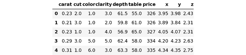

Let’s go through the code line-by-line again. First, we import the OrdinalEncoder class that encodes ordinal categorical features and initialize it. Ordinal features are variables that have natural, ordered categories as in the case of diamond quality measurements. The cut and clarity are ordinal, while color isn't. But not to complicate things, we will consider it ordinal for now.

Then, we extract the categorical feature names using the select_dtypes method of Pandas DataFrames. We chain the .columns and .tolist() attributes to get column names in a list named cats.

Then, we will use the list to transform the features we want with oe. Finally, using a neat Pandas trick with .loc, we replace the old text values with numeric ones.

Before fitting a multivariate model, we will extract the feature array X. The purpose of the diamonds dataset is to predict diamond prices given its characteristics. So, X will contain all columns but price:

X = diamonds.drop("price", axis=1)
y = diamonds[["price"]]
Now, let’s build and fit the model:
from pyod.models.iforest import IForest

# Create a model with 10000 trees
iforest = IForest(n_estimators=10000)
iforest.fit(X)  # This will take a minute

# Extract the labels
labels = iforest.labels_

The more trees IForest estimator has, the more time it takes to fit the model to the dataset.

After we have labels, we can remove the outliers from the original data:

X_outlier_free = X[labels == 0]
y_outlier_free = X[labels == 0]

>>> len(X_outlier_free)
48546

>>> # The length of the original dataset
>>> len(diamonds)
53940

The model found over 5000 outliers!

Challenges in Anomaly Detection

Anomaly detection may pose bigger challenges than other machine learning tasks because of its unsupervised nature. However, most of these challenges can be mitigated with various methods (see the next section for resources).

In outlier detection, we need to ask these two questions:

• Are the found outliers actually outliers?
• Did the model find all outliers in the data?

In supervised learning, we can easily check if the model is performing well by matching its predictions on the test data with the actual labels. But, we can’t do the same in outlier detection as there aren’t ready-made labels telling us which samples are inliers and which are outliers.

So, some or most of the +5000 outliers found from the diamonds dataset may not actually be outliers! There is no way of knowing for sure. It may have labeled some inliers as outliers while missing some actual outliers.

This problem of not knowing the contamination level (the percentage of outliers in a dataset) is the biggest one in anomaly detection. Because of it, we can’t reliably measure the performance of outlier classifiers, nor can we verify its results.

For this reason, all estimators in pyod have a parameter called contamination, which is set to 0.1 by default. As a machine learning engineer, you have to tune this parameter by yourself.

Of course, sometimes there are alternatives. For example, the IsolationForest model offered by Sklearn has an internal algorithm to find the contamination level automatically. But IsolationForest is not a silver bullet to all outlier detection problems.

Another issue in anomaly detection is the data imbalance. Anomalies are often rare compared to normal instances, causing datasets to be imbalanced. This imbalance can lead to difficulties in distinguishing between actual anomalies and irregularities within the majority class.

Addressing these issues (and much more we haven’t covered) involves choosing suitable algorithms, hyperparameter tuning, feature selection, handling class imbalance, and so on.

Summary and Next Steps

We have finished your (probably) first exposure to the fascinating world of anomaly detection. The fundamental concepts and skills in this tutorial can go a long way in exploring anomaly detection further.

To deepen your understanding, here are some resources to check out next:

• Anomaly Detection in Python course by DataCamp: covers methods and techniques more deeply discussed in this article and discusses how to address the issues presented in the last section.
• Anomaly Detection in R course by DataCamp: a course for people who prefer good-ol’ R