Everyone loves to stand out, to be different. But that’s not the quality you want in your data points as a data scientist. Divergent data points or anomalies in a dataset, are one of the most dangerous data quality issues that plague almost all data projects.

This last sentence may surprise you if you have only been working on polished open-source datasets that often come without outliers. However, real-world datasets always have some differences from the normal samples. It is your job to detect and deal with them appropriately.

In this article, you will learn the fundamental ideas of this process, which is often called anomaly detection:

1. The detrimental effect anomalies have on your project.
2. The importance of detecting anomalies.
3. Real-world applications of anomaly detection.
4. The difference between anomalies, outliers, and novelties.
5. Types of anomalies and anomaly detection methods.
6. How to build anomaly detection algorithms in Python.
7. How to deal with the challenges of anomaly detection.

By the end, you will master the fundamentals of anomaly detection and gain the confidence to mitigate the disruptive influence of outliers in your projects.

What is Anomaly Detection?

Anomaly detection, sometimes called outlier detection, is a process of finding patterns or instances in a dataset that deviate significantly from the expected or “normal behavior.”

The definition of both “normal” and anomalous data significantly varies depending on the context. Below are a few examples of anomaly detection in action.

1. Financial transactions

Normal: Routine purchases and consistent spending by an individual in London.

Outlier: A massive withdrawal from Ireland from the same account, hinting at potential fraud.

2. Network traffic in cybersecurity

Normal: Regular communication, steady data transfer, and adherence to protocol.

Outlier: Abrupt increase in data transfer or use of unknown protocols signaling a potential breach or malware.

3. Patient vital signs monitoring

Normal: Stable heart rate and consistent blood pressure

Outlier: Sudden increase in heart rate and decrease in blood pressure, indicating a potential emergency or equipment failure.

Anomaly detection includes many types of unsupervised methods to identify divergent samples. Data specialists choose them based on anomaly type, the context, structure, and characteristics of the dataset at hand. We’ll cover them in the coming sections.

Real-World Applications of Anomaly Detection

Even though we saw some examples above, let’s look at a real-life story of how anomaly detection works in finance.

Shaq O’Neal, four times NBA winner, gets traded from the Miami Heat to the Phoenix Suns. When Shaq arrives at the empty apartment provided by the Phoenix Suns, he wants to furnish his apartment immediately in the middle of the night. So, he goes to Walmart and makes the biggest purchase in Walmart history for $70,000. Or at least, he tries to; his card gets declined.

He wonders what could possibly be the problem (he can’t be broke!) At 2 am in the morning, American Express security calls him and tells him that his card was suspected as stolen because somebody was trying to make a $70,000 purchase at Walmart in Phoenix (watch the anecdote to hear the full story).

There are so many other real-world applications of anomaly detection beyond finance and fraud detection:

• Cybersecurity
• Healthcare
• Industrial equipment monitoring
• Network intrusion detection
• Energy grid monitoring
• E-commerce and user behavior analysis
• Quality control in manufacturing

Anomaly detection is deeply woven into the daily services we use and often, we don’t even notice it.

The Importance of Anomaly Detection in Data Science

Data is the most precious commodity in data science, and anomalies are the most disruptive threats to its quality. Bad data quality means bad:

• Statistical tests
• Dashboards
• Machine learning models
• Decisions

and ultimately, a compromised foundation for informed decision-making.

Anomalies distort statistical analyses by introducing non-existent patterns, leading to wrong conclusions and unreliable predictions. As they are often the extreme values in a dataset, anomalies often skew the two most important characteristics of distributions: mean and standard deviation.

As the internals of almost all machine learning models rely heavily on these two metrics, timely detection of anomalies is crucial.

Types of Anomalies

Anomaly detection encompasses two broad practices: outlier detection and novelty detection.

Outliers are abnormal or extreme data points that exist only in training data. In contrast, novelties are new or previously unseen instances compared to the original (training) data.

For example, consider a dataset of daily temperatures in a city. Most days, the temperatures range between 20°C and 30°C. However, one day, there’s a spike of 40°C. This extreme temperature is an outlier as it significantly deviates from the usual daily temperature range.

Now, imagine that the city installs a new, more accurate weather monitoring station. As a result, the dataset starts consistently recording slightly higher temperatures, ranging from 25°C to 35°C. This sustained increase in temperatures is a novelty, representing a new pattern introduced by the improved monitoring system.

Anomalies, on the other hand, is a broad term for both outliers and novelties. It can be used to define any abnormal instance in any context.

Identifying the type of anomalies is crucial as it allows you to choose the right algorithm to detect them.

Types of Outliers

As there are two types of anomalies, there are two types of outliers as well: univariate and multivariate. Depending on the type, we will use different detection algorithms.

1. Univariate outliers exist in a single variable or feature in isolation. Univariate outliers are extreme or abnormal values that deviate from the typical range of values for that specific feature.
2. Multivariate outliers are found by combining the values of multiple variables at the same time.

For example, consider a dataset of housing prices in a neighborhood. Most houses cost between $200,000 and $400,000, but there is House A with an exceptionally high price of $1,000,000. When we analyze only the price, House A is a clear outlier.

Now, let’s add two more variables to our dataset: the square footage and the number of bedrooms. When we consider the square footage, the number of bedrooms, and the price, it’s House B that looks odd:

• It has half the square footage of the mean house price.
• It has only one bedroom.
• It costs the top of the range $380.000.

When we look at these variables individually, they seem ordinary. Only when we put them together do we find out that House B is a clear multivariate outlier.

Anomaly Detection Methods And When to Use Each One

Anomaly detection algorithms differ depending on the type of outliers and the structure in the dataset.

For univariate outlier detection, the most popular methods are:

1. Z-score (standard score): the z-score measures how many standard deviations a data point is away from the mean. Generally, instances with a z-score over 3 are chosen as outliers.
2. Interquartile range (IQR): The IQR is the range between the first quartile (Q1) and the third quartile (Q3) of a distribution. When an instance is beyond Q1 or Q3 for some multiplier of IQR, they are considered outliers. The most common multiplier is 1.5, making the outlier range [Q1–1.5 * IQR, Q3 + 1.5 * IQR].
3. Modified z-scores: similar to z-scores, but modified z-scores use the median and a measure called Median Absolute Deviation (MAD) to find outliers. Since mean and standard deviation are easily skewed by outliers, modified z-scores are generally considered more robust.

For multivariate outliers, we generally use machine learning algorithms. Because of their depth and strength, they are able to find intricate patterns in complex datasets:

1. Isolation Forest: uses a collection of isolation trees (similar to decision trees) that recursively divide complex datasets until each instance is isolated. The instances that get isolated the quickest are considered outliers.
2. Local Outlier Factor (LOF): LOF measures the local density deviation of a sample compared to its neighbors. Points with significantly lower density are chosen as outliers.
3. Clustering techniques: techniques such as k-means or hierarchical clustering divide the dataset into groups. Points that don’t belong to any group or are in their own little clusters are considered outliers.
4. Angle-based Outlier Detection (ABOD): ABOD measures the angles between individual points. Instances with odd angles can be considered outliers.

Apart from the type of anomalies, you should consider dataset characteristics and project constraints. For example, Isolation Forest works well on almost any dataset but it is slower and computation-heavy as it is an ensemble method. In comparison, LOF is very fast in training but may not perform as well as Isolation Forest.

You can see a comparison of the most common Anomaly Detection algorithms on 55 datasets from Python Outlier Detection (PyOD) package.

Building an Anomaly Detection Model in Python

Like virtually any task, there are many libraries in Python to perform anomaly detection. The best contenders are:

• Python Outlier Detection (PyOD)
• Scikit-learn

While scikit-learn offers five classic machine learning algorithms (you can use them for both univariate and multivariate outliers), PyOD includes over 30 algorithms, from simple methods such as MAD to complex deep learning models. You can also use TensorFlow or PyTorch for custom models, but they are beyond the scope of this article.

Univariate anomaly detection

I prefer pyod for its rich library of algorithms and an API consistent with sklearn. It takes just a few lines of code to find and extract outliers from a dataset using PyOD. Here is an example of using MAD on a univariate dataset:

import pandas as pd
import seaborn as sns
from pyod.models.mad import MAD

# Load a sample dataset
diamonds = sns.load_dataset("diamonds")
# Extract the feature we want
X = diamonds[["price"]]

# Initialize and fit a model
mad = MAD().fit(X)

# Extract the outlier labels
labels = mad.labels_

>>> pd.Series(labels).value_counts()
0    49708
1     4232
Name: count, dtype: int64

Let’s go through the code line-by-line. First, we load the necessary libraries for data manipulation, loading a dataset and pyod for the outlier detection model. Then, after loading the Diamonds dataset built into Seaborn, we extract the diamond prices.

Then, we initialize and fit a Median Absolute Deviation (MAD) model to X in a single line. Next, we extract the inlier and outlier labels using the labels_ attribute of mad into labels.

When we print the value counts of labels at the end, we see that 49708 belongs to category 0 (inliers) while 4232 belongs to 1 (outliers). If we want to remove the outliers from the original dataset, we can use pandas subsetting on diamonds:

outlier_free = diamonds[labels == 0]

>>> len(outlier_free)
49708

labels == 0 creates an array of True/False values (boolean array) where True denotes an inlier.

Multivariate anomaly detection

The process of creating a multivariate anomaly detection model is also the same. But multivariate outlier detection requires extra processing steps if categorical features are present:

>>> diamonds.info()
<class 'pandas.core.frame.DataFrame'>
RangeIndex: 53940 entries, 0 to 53939
Data columns (total 10 columns):
#   Column   Non-Null Count  Dtype  
---  ------   --------------  -----  
0   carat    53940 non-null  float64
1   cut      53940 non-null  category
2   color    53940 non-null  category
3   clarity  53940 non-null  category
4   depth    53940 non-null  float64
5   table    53940 non-null  float64
6   price    53940 non-null  int64  
7   x        53940 non-null  float64
8   y        53940 non-null  float64
9   z        53940 non-null  float64
dtypes: category(3), float64(6), int64(1)
memory usage: 3.0 MB

Since pyod expects all features to be numeric, we need to encode categorical variables. We will use Sklearn to do so:

from sklearn.preprocessing import OrdinalEncoder

# Initialize the encoder
oe = OrdinalEncoder()

# Extract the categorical feature names
cats = diamonds.select_dtypes(include="category").columns.tolist()

# Encode the categorical features
cats_encoded = oe.fit_transform(diamonds[cats])

# Replace the old values with encoded values
diamonds.loc[:, cats] = cats_encoded

>>> diamonds.head()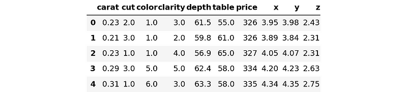

Let’s go through the code line-by-line again. First, we import the OrdinalEncoder class that encodes ordinal categorical features and initialize it. Ordinal features are variables that have natural, ordered categories as in the case of diamond quality measurements. The cut and clarity are ordinal, while color isn't. But not to complicate things, we will consider it ordinal for now.

Then, we extract the categorical feature names using the select_dtypes method of Pandas DataFrames. We chain the .columns and .tolist() attributes to get column names in a list named cats.

Then, we will use the list to transform the features we want with oe. Finally, using a neat Pandas trick with .loc, we replace the old text values with numeric ones.

Before fitting a multivariate model, we will extract the feature array X. The purpose of the diamonds dataset is to predict diamond prices given its characteristics. So, X will contain all columns but price:

X = diamonds.drop("price", axis=1)
y = diamonds[["price"]]
Now, let’s build and fit the model:
from pyod.models.iforest import IForest

# Create a model with 10000 trees
iforest = IForest(n_estimators=10000)
iforest.fit(X)  # This will take a minute

# Extract the labels
labels = iforest.labels_

The more trees IForest estimator has, the more time it takes to fit the model to the dataset.

After we have labels, we can remove the outliers from the original data:

X_outlier_free = X[labels == 0]
y_outlier_free = X[labels == 0]

>>> len(X_outlier_free)
48546

>>> # The length of the original dataset
>>> len(diamonds)
53940

The model found over 5000 outliers!

Challenges in Anomaly Detection

Anomaly detection may pose bigger challenges than other machine learning tasks because of its unsupervised nature. However, most of these challenges can be mitigated with various methods (see the next section for resources).

In outlier detection, we need to ask these two questions:

• Are the found outliers actually outliers?
• Did the model find all outliers in the data?

In supervised learning, we can easily check if the model is performing well by matching its predictions on the test data with the actual labels. But, we can’t do the same in outlier detection as there aren’t ready-made labels telling us which samples are inliers and which are outliers.

So, some or most of the +5000 outliers found from the diamonds dataset may not actually be outliers! There is no way of knowing for sure. It may have labeled some inliers as outliers while missing some actual outliers.

This problem of not knowing the contamination level (the percentage of outliers in a dataset) is the biggest one in anomaly detection. Because of it, we can’t reliably measure the performance of outlier classifiers, nor can we verify its results.

For this reason, all estimators in pyod have a parameter called contamination, which is set to 0.1 by default. As a machine learning engineer, you have to tune this parameter by yourself.

Of course, sometimes there are alternatives. For example, the IsolationForest model offered by Sklearn has an internal algorithm to find the contamination level automatically. But IsolationForest is not a silver bullet to all outlier detection problems.

Another issue in anomaly detection is the data imbalance. Anomalies are often rare compared to normal instances, causing datasets to be imbalanced. This imbalance can lead to difficulties in distinguishing between actual anomalies and irregularities within the majority class.

Addressing these issues (and much more we haven’t covered) involves choosing suitable algorithms, hyperparameter tuning, feature selection, handling class imbalance, and so on.

Summary and Next Steps

We have finished your (probably) first exposure to the fascinating world of anomaly detection. The fundamental concepts and skills in this tutorial can go a long way in exploring anomaly detection further.

To deepen your understanding, here are some resources to check out next:

• Anomaly Detection in Python course by DataCamp: covers methods and techniques more deeply discussed in this article and discusses how to address the issues presented in the last section.
• Anomaly Detection in R course by DataCamp: a course for people who prefer good-ol’ R