VLOOKUP() in Google Sheets: zo gebruik je het + voorbeelden

VLOOKUP() is een functie in Google Sheets die een waarde in een kolom zoekt en een overeenkomende waarde uit een andere kolom in dezelfde rij retourneert. Je geeft op wat je wilt vinden, waar je moet zoeken, en het haalt de gegevens op die je nodig hebt.

Dit is vooral handig bij grote datasets waarbij handmatig zoeken en matchen te lang zou duren. Maar elke keer dat je twee tabellen met gegevens aan elkaar wilt koppelen op basis van een gedeelde waarde, is VLOOKUP() de aangewezen functie.

In deze gids leer je de syntaxis, hoe je de functie stap voor stap gebruikt, waardoor onjuiste resultaten kunnen ontstaan, en wanneer je beter kunt kiezen voor alternatieven zoals INDEX MATCH() of XLOOKUP().

Wat is de syntaxis van VLOOKUP() in Google Sheets?

De syntaxis van VLOOKUP() is:

=VLOOKUP(search_key, range, index, [is_sorted])

Hierbij geldt: 

• search_key is de waarde die je wilt zoeken

• range is de tabel waarin gezocht wordt

• index is het kolomnummer waaruit je het resultaat wilt terugkrijgen

• [is_sorted] bepaalt of je een exacte overeenkomst wilt of niet

Hoe doe je een VLOOKUP() in Google Sheets?

Zo voer je een VLOOKUP() uit in Google Sheets:

1. Bepaal welke waarde je wilt opzoeken: Dit kan een ID, naam of een andere unieke waarde zijn.

2. Bepaal je tabelbereik: Zorg dat de kolom met je zoekwaarde de eerste kolom in dat bereik is.

3. Kies welke gegevens je wilt terugkrijgen: Dit is de kolom met het resultaat (bijv. naam, prijs, status).

4. Voer de VLOOKUP()-formule in een nieuwe cel in: Verwijs naar je zoekwaarde, tabelbereik en de kolom die je wilt retourneren.

5. Gebruik exacte of benaderende overeenkomst (FALSE of TRUE): In de meeste gevallen wil je een exacte overeenkomst om verkeerde resultaten te voorkomen (daarover later meer).

Als je deze tabel hebt:

En je wilt de naam bij ID 102 vinden, gebruik dan:

=VLOOKUP(102, A2:B4, 2, FALSE)

Dit vertelt Google Sheets om:

• 102 in kolom A te zoeken
• De waarde uit kolom B te retourneren
• Een exacte overeenkomst te geven

Als resultaat krijg je Sarah.

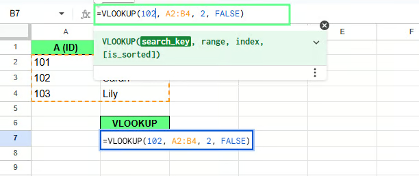
Voorbeeld van VLOOKUP(). Afbeelding door auteur.

Hoe VLOOKUP() werkt (stap-voor-stap-logica)

VLOOKUP() volgt een eenvoudig verticaal zoekproces. Het begint altijd met de eerste kolom van je geselecteerde bereik en scant vervolgens omlaag, rij voor rij, totdat het de eerste overeenkomst vindt.

Zodra die overeenkomst is gevonden, blijft het in dezelfde rij. Vervolgens gaat het naar de door jou opgegeven kolom en retourneert die waarde.

Zo werkt het stap voor stap:

• Begint in de eerste kolom van het bereik
• Zoekt naar beneden in de kolom
• Vindt de eerste overeenkomende waarde
• Gaat in dezelfde rij opzij
• Retourneert gegevens uit de opgegeven kolom

Stel dat je de functietitel wilt vinden voor medewerker-ID E1007. Gebruik hiervoor de volgende formule:

=VLOOKUP("E1007", A:G, 5, FALSE)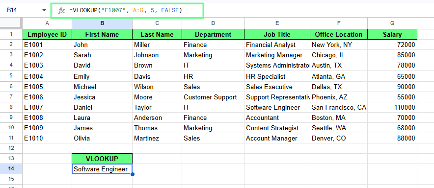

VLOOKUP() in Google Sheets. Afbeelding door auteur.

Deze formule:

• Zoekt E1007 in kolom A

• Gaat in dezelfde rij opzij

• Retourneert kolom 5 (Functietitel)

• Geeft als resultaat Software Engineer.

Let op: VLOOKUP() kan alleen van links naar rechts zoeken. Als je zoekkolom niet de eerste kolom in het bereik is, werkt de functie niet. In dat geval moet je je gegevens herschikken of een andere functie gebruiken. Daar komen we later op terug.

Exacte versus benaderende overeenkomst in VLOOKUP()

Een exacte overeenkomst retourneert alleen een resultaat wanneer de waarde identiek is. Een benaderende overeenkomst retourneert de dichtstbijzijnde beschikbare waarde als er geen exacte overeenkomst is, meestal op basis van gesorteerde gegevens.

In VLOOKUP() wordt dit bepaald door het laatste argument. Dat laatste argument, FALSE of TRUE, is waar de meesten de fout in gaan, omdat TRUE onschuldig lijkt en dat niet is.

• FALSE betekent alleen een exacte overeenkomst. Als de waarde er niet is, krijg je #N/A, wat eigenlijk nuttig is. 
• TRUE retourneert de dichtstbijzijnde lagere waarde wanneer er geen exacte overeenkomst bestaat. Dat klinkt als een terugvaloptie, maar is eerder een stille, verkeerde uitkomst. Het gaat er ook vanuit dat je gegevens gesorteerd zijn. Als dat niet zo is, is het resultaat ongedefinieerd. 

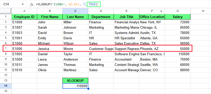
Ik zou zeggen: gebruik TRUE alleen voor getrapte opzoekingen, zoals belastingschijven of cijferbanden, waar benaderen per ontwerp het juiste gedrag is. Voor alles daarbuiten: gebruik FALSE.

Exacte overeenkomst (FALSE)

Dit vertelt VLOOKUP(): “Geef alleen een resultaat terug als je precies deze waarde vindt.” Bijvoorbeeld, deze formule =VLOOKUP("E1005", A:G, 7, FALSE) zoekt naar E1005, retourneert het salaris uit kolom 7 en geeft als resultaat 90000.

Bestaat de waarde niet, dan krijg je een #N/A-fout. 

Exacte overeenkomst in VLOOKUP(). Afbeelding door auteur.

Benaderende overeenkomst (TRUE)

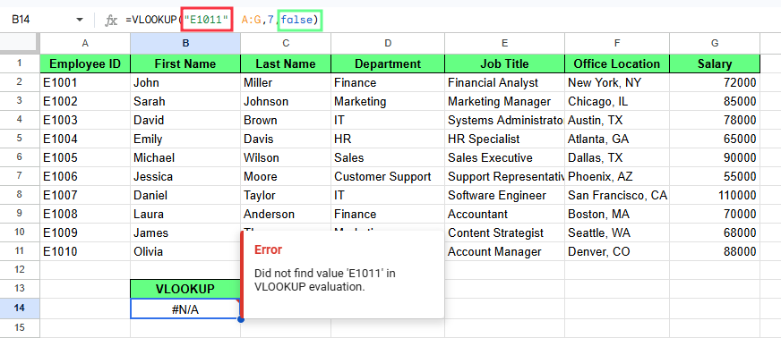
Dit vertelt VLOOKUP(): “Als je geen exacte overeenkomst vindt, retourneer de dichtstbijzijnde waarde eronder.” Dat klinkt handig — soms is het dat ook, maar soms geeft het je stilletjes een verkeerd antwoord.

Bijvoorbeeld, E1011 bestaat niet in onze dataset. De laatste medewerker-ID is E1010. Dus als je deze formule gebruikt =VLOOKUP("E1011", A:G, 7, TRUE), zal VLOOKUP() geen fout retourneren. In plaats daarvan geeft het de waarde voor de dichtstbijzijnde lagere overeenkomst, namelijk E1010. De cel toont 88000.

Dus ook al ontbreekt E1011, VLOOKUP() geeft toch een resultaat omdat TRUE een benaderende overeenkomst toestaat.

Benaderende overeenkomst in VLOOKUP(). Afbeelding door auteur.

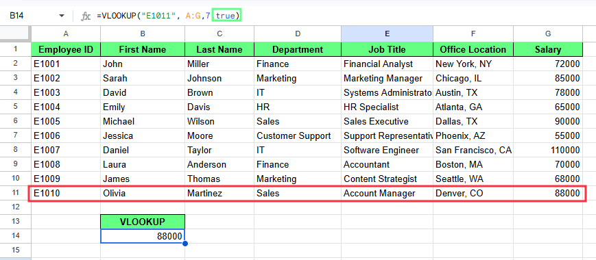
Stel je nu voor dat dezelfde gegevens niet op volgorde staan, en ik voer de beschikbare medewerker-ID in de formule in, zoals: =VLOOKUP("E1011", A:G, 7, TRUE).

Deze keer retourneert de formule een onjuist salaris omdat de zoekkolom niet is gesorteerd, en de benaderende overeenkomst van gesorteerde gegevens afhankelijk is.

VLOOKUP() met benaderende overeenkomst geeft een fout door een niet-gesorteerde lijst. Afbeelding door auteur.

Veelvoorkomende fouten in VLOOKUP() en hoe je ze oplost

Laten we enkele van de meest voorkomende problemen met VLOOKUP() bekijken en hoe je ze oplost: 

#N/A-fout

Een #N/A-fout betekent dat VLOOKUP() de gevraagde waarde niet kon vinden.

Stel, je hebt deze formule: =VLOOKUP("E9999", A:G, 7, FALSE)

 Als E9999 niet in de eerste kolom van het bereik staat, geeft de formule #N/A terug.

Dit kan ook gebeuren als de waarde anders is getypt in het blad, bijvoorbeeld met extra spaties of problemen met tekstopmaak.

Zo los je het op:

• Zorg dat de waarde in de eerste kolom van het bereik staat

• Gebruik waar mogelijk de juiste celverwijzing in plaats van de waarde handmatig te typen

• Voeg aanhalingstekens toe als je een tekstwaarde hardcodeert

• Verwijder spaties aan het begin of einde uit de gegevens

• Gebruik FALSE alleen wanneer je een exacte overeenkomst nodig hebt 

Verkeerde kolomindex

De kolomindex vertelt VLOOKUP() uit welke kolom binnen het geselecteerde bereik geretourneerd moet worden. Als het indexgetal te groot is, geeft de formule #REF! terug.

Deze =VLOOKUP("E1005", A:G, 8, FALSE) geeft #REF! omdat het bereik A:G slechts 7 kolommen heeft.

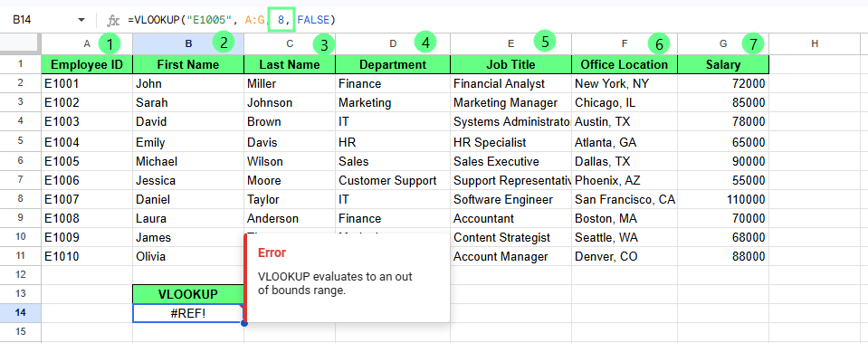
Verkeerde kolomindex geeft een fout. Afbeelding door auteur.

Je kunt ook het verkeerde resultaat krijgen als het kolomnummer wel geldig is maar naar de verkeerde kolom verwijst.

Bijvoorbeeld:

=VLOOKUP("E1005", A:G, 5, FALSE)

Dit retourneert de functietitel, niet het salaris.

Zo los je het op:

• Tel kolommen vanaf de eerste kolom van je geselecteerde bereik
• Controleer of het kolomnummer overeenkomt met de waarde die je wilt retourneren
• Zorg dat de kolom binnen het bereik bestaat

Problemen met benaderende overeenkomst

Als je TRUE gebruikt, zoekt VLOOKUP() naar de dichtstbijzijnde lagere overeenkomst in plaats van een exacte te vereisen.

Als je =VLOOKUP("E1011", A:G, 7, TRUE) typt en er is geen E1011 in de dataset, dan retourneert de formule in plaats van een fout 88000, wat bij E1010 hoort.

Dat resultaat kan correct lijken, maar het is geen exacte overeenkomst.

Zo los je het op:

• Gebruik FALSE als je een exact resultaat nodig hebt

• Gebruik TRUE alleen wanneer de gegevens gesorteerd zijn en een benaderend resultaat acceptabel is

Bereikproblemen

VLOOKUP() kan ook ophouden met werken wanneer het geselecteerde bereik niet past bij wat de formule probeert te doen.

Zo geeft =VLOOKUP("E1005", A:C, 7, FALSE) #REF! omdat het bereik A:C slechts 3 kolommen heeft, maar de formule om kolom 7 vraagt.

Een ander veelvoorkomend probleem treedt op wanneer de zoekkolom niet de eerste kolom in het bereik is.

Zie deze formule:

=VLOOKUP("E1005", B:G, 7, FALSE)

Hier is de eerste kolom in het bereik kolom B, niet kolom A. Omdat VLOOKUP() alleen de eerste kolom van het geselecteerde bereik doorzoekt, kan het E1005 niet vinden.

Zo los je het op:

• Zorg dat de zoekkolom de eerste kolom in het bereik is
• Zorg dat het bereik de kolom bevat die je wilt retourneren
• Controleer het geselecteerde bereik goed voordat je de formule afrondt

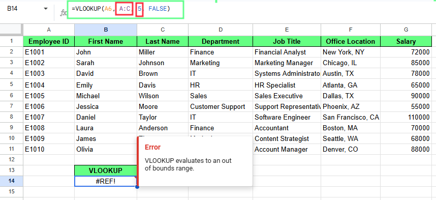
Verkeerd bereik geeft een fout. Afbeelding door auteur.

VLOOKUP() over meerdere tabbladen in Google Sheets

Je kunt VLOOKUP() gebruiken om gegevens uit een ander tabblad op te halen door de bladnaam vóór het bereik te zetten.

Het formaat ziet er zo uit:

=VLOOKUP(search_key, SheetName!range, index, FALSE)

Het deel SheetName! vertelt de formule in welk tabblad moet worden gezocht.

Stel dat je gegevens zijn opgeslagen in een tabblad genaamd Employees en je werkt in een ander tabblad. Om de afdeling voor medewerker-ID E1005 te vinden, gebruik je:

=VLOOKUP("E1005", Employees!A:G, 4, FALSE)

Hier:

• Employees!A:G zoekt in het tabblad Employees

• 4 retourneert de kolom Department

De formule retourneert de afdeling voor E1005.

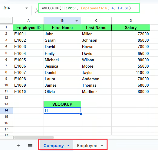
Verwijzen naar een ander tabblad in VLOOKUP(). Afbeelding door auteur.

Als bladnamen spaties bevatten

Als de bladnaam spaties bevat, zet deze dan tussen enkele aanhalingstekens zoals dit: 

=VLOOKUP("E1005", 'Employee Data'!A:G, 7, FALSE)

Zonder de aanhalingstekens werkt de formule niet.

VLOOKUP() vs. INDEX MATCH in Google Sheets

VLOOKUP() zoekt in een vaste kolom en retourneert gegevens op basis van positie, terwijl INDEX MATCH waarden rechtstreeks vindt met rij- en kolomverwijzingen, waardoor het blijft werken zelfs als de tabelstructuur verandert.

VLOOKUP: snel te schrijven, snel stuk

Je zag al dat =VLOOKUP("E1005", A:G, 7, FALSE) het salaris voor E1005 vindt. 

Dat werkt goed als:

• De zoekkolom links staat
• De tabelstructuur niet verandert

Problemen ontstaan zodra de structuur verandert.

Bijvoorbeeld:

• Je voegt een nieuwe kolom in
• De salaris-kolom verschuift van 7 naar 8
• De formule gebruikt nog steeds 7

Nu retourneert die zonder foutmelding de verkeerde waarde.

INDEX MATCH: langer, maar stabiel

Bekijk nu dezelfde opzoekactie met INDEX MATCH:

=INDEX(G:G, MATCH("E1005", A:A, 0))

Hierbij:

• MATCH() vindt de positie van E1005 in kolom A

• INDEX() retourneert de waarde uit kolom G op die positie

Deze methode is niet afhankelijk van kolomnummers en blijft dus werken als de tabel verandert.

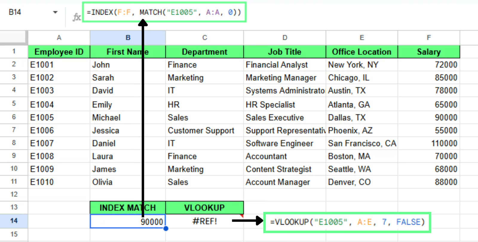
INDEX MATCH gaat beter met de gegevens om dan VLOOKUP(). Afbeelding door auteur.

Wanneer het echt helpt

Gebruik INDEX MATCH wanneer je gegevens niet van links naar rechts geordend zijn. Stel dat kolom A medewerker-ID bevat en kolom C de achternaam. Als je op achternaam wilt zoeken en medewerker-ID wilt retourneren, is dit een zoekactie van rechts naar links.

VLOOKUP() kan dit niet zonder de tabel te wijzigen, maar INDEX MATCH kan het direct afhandelen:

=INDEX(A:A, MATCH("Wilson", C:C, 0))

Je hoeft je gegevens niet te herschikken.

VLOOKUP() vs XLOOKUP in Google Sheets

VLOOKUP() zoekt binnen een vaste structuur en heeft beperkingen, terwijl XLOOKUP() in elke richting kan zoeken. Deze functie is in 2022 aan Google Sheets toegevoegd en is in veel gevallen nu de betere optie.

Stel dat je de medewerker-ID wilt vinden met de achternaam Wilson. Dit is een zoekactie van rechts naar links. VLOOKUP() kan dit niet zonder de tabel te herschikken, maar XLOOKUP() kan het wel:

=XLOOKUP("Wilson", C:C, A:A)

Deze formule:

• Zoekt in Achternaam (kolom C)
• Retourneert Medewerker-ID (kolom A)

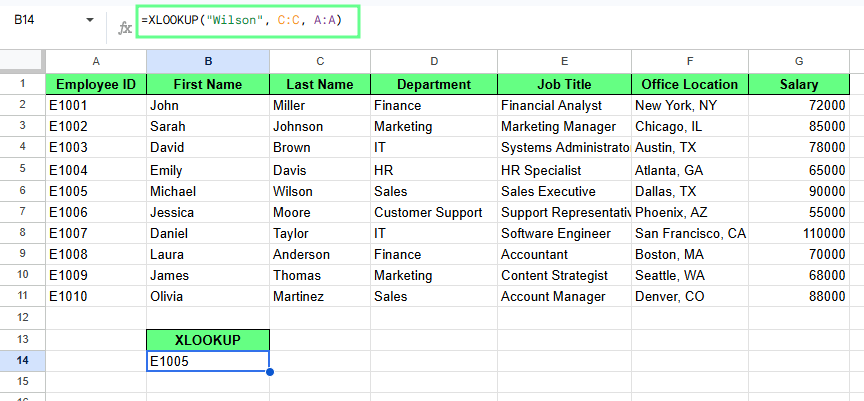
XLOOKUP() in Google Sheets. Afbeelding door auteur.

XLOOKUP() is beter omdat het: 

• In elke richting werkt (links of rechts)
• Geen kolomnummers gebruikt
• Standaard exacte overeenkomsten retourneert
• Aangepaste uitvoer toestaat wanneer er geen overeenkomst is 

Tot slot 

Als ik één advies mocht geven: bouw VLOOKUP() in een echt spreadsheet waar je daadwerkelijk om geeft, in plaats van in een oefenblad. Fouten komen anders binnen wanneer de data belangrijk is. Je herinnert je wel waarom FALSE bestaat zodra TRUE je stilletjes iemands verkeerde salaris geeft.

Als je er eenmaal vertrouwd mee bent, probeer dan verschillende matchtypes, pas je bereiken aan en let op wanneer de resultaten niet meer logisch zijn. Dat is meestal het moment waarop een flexibelere optie zoals INDEX MATCH() of XLOOKUP() meer zin heeft.