ONNX : Entraînez-vous dans n'importe quel cadre, déployez sur n'importe quel matériel

Vous avez donc formé un modèle dans PyTorch, mais votre système de production utilise TensorFlow. Est-il nécessaire de réécrire tout le contenu à partir de zéro ?

Non, ce n'est pas nécessaire.

L'interopérabilité des modèles peut poser des difficultés aux ingénieurs en apprentissage automatique. Différents frameworks utilisent différents formats, et la conversion entre ceux-ci peut endommager votre modèle ou entraîner un comportement inattendu. Vous ne souhaitez pas cela, mais vous ne souhaitez pas non plus conserver plusieurs versions du même modèle.

ONNX (Open Neural Network Exchange) résout ce problème en fournissant un format universel pour les modèles d'apprentissage automatique. Il vous permet de vous former dans un cadre et de déployer dans un autre sans réécrire de code ni gérer de bugs.

Dans cet article, je vais vous expliquer comment convertir des modèles au format ONNX, exécuter des inférences avec ONNX Runtime, optimiser des modèles pour la production et les déployer sur diverses plateformes, des appareils périphériques aux serveurs cloud.

Premiers pas avec ONNX

Il est nécessaire de configurer votre environnement de développement avant de pouvoir utiliser ONNX.

Dans cette section, je vous présenterai tout ce dont vous avez besoin, des exigences logicielles à la création d'un espace de travail propre et reproductible. Je vais vous expliquer comment installer ONNX et ONNX Runtime sur Windows, Linux et macOS.

Conditions préalables

ONNX est compatible avec tous les principaux systèmes d'exploitation.

Il est nécessaire que Python 3.8 ou une version supérieure soit installé sur votre ordinateur. Voilà pour les notions de base. ONNX prend en charge l'interface binaire d'application ( ABI3 ) de Python, ce qui signifie que vous pouvez utiliser des paquets binaires précompilés sans avoir à compiler à partir du code source.

Voici ce que vous allez installer :

• uv (Veuillez le télécharger à partir de astral.sh/uv)

• Python 3.8+ (uv s'en charge pour vous)

• pip (fourni avec l'uv)

Si vous souhaitez en savoir plus sur le fonctionnement d'uv et les raisons pour lesquelles il devrait être votre choix privilégié, veuillez consulter notre guide sur le gestionnaire de paquets Python le plus rapide.

Pour les utilisateurs Windows, vous pouvez installer uv à l'aide de PowerShell :

powershell -c "irm <https://astral.sh/uv/install.ps1> | iex"

Si vous rencontrez une erreur liée à la stratégie d'exécution, veuillez d'abord exécuter PowerShell en tant qu'administrateur.

Les utilisateurs Linux peuvent installer uv à l'aide de cette commande shell :

curl -LsSf <https://astral.sh/uv/install.sh> | sh

Ceci est compatible avec toutes les distributions Linux.

Enfin, les utilisateurs de macOS peuvent installer uv à l'aide de Homebrew ou d'une commande curl :

brew install uv

# or

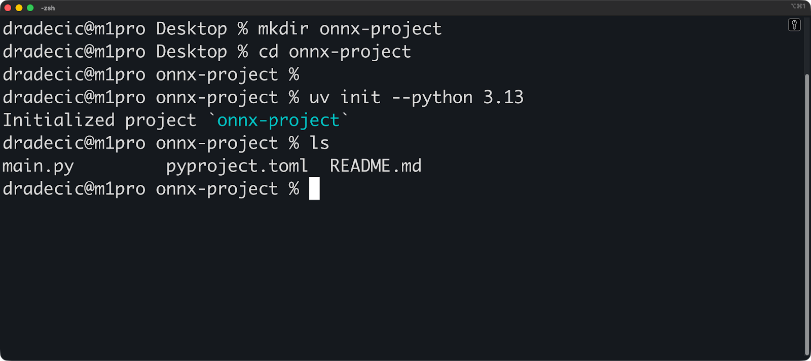
curl -LsSf <https://astral.sh/uv/install.sh> | sh

Configuration de l'environnement

Voici comment configurer un projet avec uv :

mkdir onnx-project
cd onnx-project

# Initialize a uv project with Python 3.10
uv init --python 3.13

uv crée un répertoire .venv et un fichier pyproject.toml. L'environnement virtuel s'active automatiquement lorsque vous exécutez des commandes via uv.

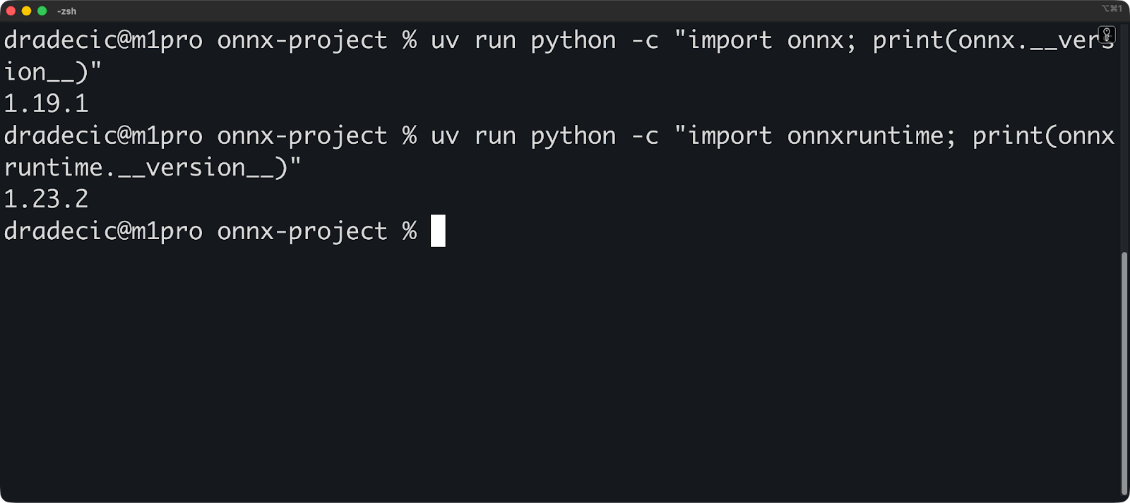
Veuillez maintenant installer ONNX et ONNX Runtime :

uv add onnx onnxruntime

# Verify the installation
uv run python -c "import onnx; print(onnx.__version__)"
uv run python -c "import onnxruntime; print(onnxruntime.__version__)"

Les commandes de vérification devraient afficher les numéros de version :

Vos dépendances sont déjà épinglées. uv enregistre automatiquement toutes les versions des paquets sur uv.lock. Cela rend vos builds reproductibles : n'importe qui peut recréer votre environnement exact en exécutant uv sync.

Voici à quoi ressemble votre fichier pyproject.toml:

[project]
name = "onnx-project"
version = "0.1.0"
description = "Add your description here"
readme = "README.md"
requires-python = ">=3.13"
dependencies = [
    "onnx>=1.19.1",
    "onnxruntime>=1.23.2",
]

Et voilà, l'environnement est configuré. Commençons par les principes fondamentaux.

Comprendre les principes fondamentaux d'ONNX

Il est important de comprendre le fonctionnement d'ONNX avant de commencer à convertir des modèles.

Dans cette section, je vais décrire le format ONNX et expliquer son architecture basée sur des graphes. Je vais vous présenter le contenu d'un fichier ONNX et la manière dont les données y circulent.

Le format de modèle ONNX

Un modèle ONNX est un fichier qui contient la structure et les poids de votre réseau neuronal.

Considérez cela comme un plan directeur. Le fichier décrit les opérations à effectuer, leur ordre d'exécution et les paramètres à utiliser. Vos poids entraînés sont stockés avec ce plan, de sorte que le modèle est prêt à fonctionner sans fichiers supplémentaires.

ONNX a été lancé en 2017 dans le cadre d'une collaboration entre Microsoft et Facebook (aujourd'hui Meta). L'objectif était simple : éviter de réécrire les modèles à chaque changement de framework. PyTorch, TensorFlow et d'autres frameworks ont continué à s'améliorer, mais les modèles ne pouvaient pas passer de l'un à l'autre sans conversion manuelle.

ONNX a modifié cette situation. La version 1.0 prenait en charge les opérations de base pour la vision par ordinateur et les réseaux neuronaux simples. Aujourd'hui, ONNX prend en charge les transformateurs, les grands modèles linguistiques et les architectures complexes qui n'existaient pas en 2017.

Il utilise les Protocol Buffers (protobuf) pour sérialiser ces données. Protobuf est un format binaire développé par Google pour le stockage et la transmission efficaces des données. Il est beaucoup plus rapide à lire et à écrire que JSON ou XML, et les fichiers sont plus petits. Tout le monde y gagne.

Voici ce que contient un modèle ONNX :

• Graphique : L'architecture du réseau
• Poids : Paramètres du modèle formé
• Métadonnées : Informations sur la version, nom du fabricant et documentation du modèle
• Version Opset : Quelles sont les opérations disponibles ?

La version de l'opset est importante. ONNX évolue au fil du temps, et continue d'ajouter de nouvelles opérations et d'améliorer celles qui existent déjà. Votre fichier modèle indique la version d'opset qu'il utilise, de sorte que le runtime sait comment l'exécuter.

Concepts clés et architecture

ONNX représente votre modèle sous la forme d'un graphe computationnel.

Un graphe comporte des nœuds et des arêtes. Les nœuds représentent des opérations (telles que la multiplication matricielle ou les fonctions d'activation), et les arêtes sont des tenseurs (vos données) circulant entre ces opérations. Voici comment ONNX décrit « multiplier ces matrices, puis appliquer ReLU, puis multiplier à nouveau ».

Voici un exemple simple :

import onnx
from onnx import helper, TensorProto

# Create input and output tensors
input_tensor = helper.make_tensor_value_info(
    "input", TensorProto.FLOAT, [1, 3, 224, 224]
)
output_tensor = helper.make_tensor_value_info("output", TensorProto.FLOAT, [1, 1000])

# Create a node (operation)
node = helper.make_node(
    "Relu",  # Operation type
    ["input"],  # Input edges 
    ["output"],  # Output edges
)

# Create the graph
graph = helper.make_graph(
    [node],  # List of nodes
    "simple_model",  # Graph name
    [input_tensor],  # Inputs
    [output_tensor],  # Outputs
)

# Create the model
model = helper.make_model(graph)
onnx.save(model, "simple_model.onnx")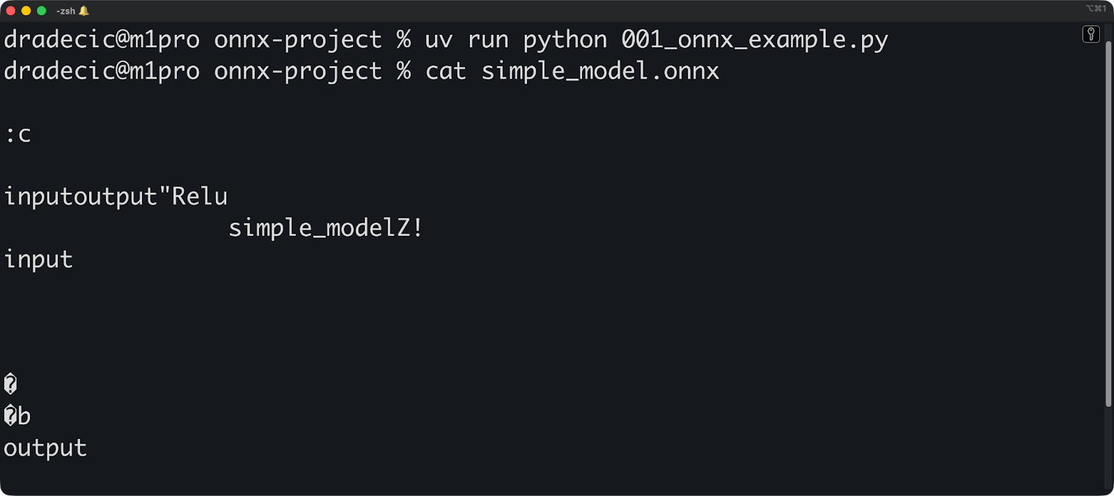

Chaque nœud effectue une opération. Le type d'opération (tel que Relu, Conv ou MatMul) provient de l'ensemble d'opérateurs ONNX. Il n'est pas possible de créer des noms d'opérations arbitraires ; ceux-ci doivent exister dans la version de l'opset que vous utilisez.

Les arêtes relient les nœuds et transportent les tenseurs. Un tenseur possède une forme et un type de données. Lorsque vous définissez [1, 3, 224, 224], vous indiquez que « ce tenseur possède 4 dimensions avec ces tailles ». Le runtime utilise ces informations pour allouer de la mémoire et valider le graphe.

Le graphique suit une seule direction. Les données entrent par les nœuds d'entrée, passent par les opérations et sortent par les nœuds de sortie. Les cycles ne sont pas autorisés - ONNX ne prend pas directement en charge les connexions récurrentes. Il est nécessaire de dérouler les boucles ou d'utiliser des opérations spécifiques conçues pour les séquences.

Cette structure graphique permet l'interopérabilité des cadres. PyTorch fonctionne selon le principe de l'exécution immédiate, TensorFlow utilise des graphes statiques et scikit-learn a une abstraction complètement différente. Cependant, ils peuvent tous exporter vers le même format graphique.

Le graphique permet également une optimisation partagée. Un optimiseur ONNX peut fusionner des opérations (combiner plusieurs nœuds en un seul), éliminer le code mort (supprimer les nœuds inutilisés) ou remplacer les opérations lentes par des équivalents plus rapides. Ces optimisations sont efficaces quel que soit le framework utilisé pour créer le modèle.

À présent, permettez-moi de vous présenter en détail la conversion de modèles au format ONNX.

Conversion des modèles au format ONNX

Dans cette section, je vais vous expliquer comment exporter des modèles depuis PyTorch, TensorFlow et scikit-learn. Je vais vous guider tout au long du processus de conversion et vous montrer comment vérifier que votre modèle fonctionne correctement après la conversion.

Assistance et outils relatifs au cadre

ONNX prend en charge les frameworks d'apprentissage automatique les plus courants.

PyTorch intègre une fonctionnalité d'exportation ONNX via torch.onnx.export(). Il s'agit du convertisseur le plus abouti, car PyTorch et ONNX sont tous deux gérés par Meta.

TensorFlow utilise tf2onnx pour la conversion. Il s'agit d'une bibliothèque distincte qui convertit les graphiques TensorFlow au format ONNX. Veuillez l'installer à l'aide de l' uv add tf2onnx, et vous serez prêt à commencer.

scikit-learn effectue la conversion via skl2onnx. Cette bibliothèque gère les modèles traditionnels d'apprentissage automatique tels que les forêts aléatoires, la régression linéaire et les SVM. Les frameworks d'apprentissage profond bénéficient d'une attention accrue, mais les modèles scikit-learn sont tout aussi performants.

Ces trois frameworks sont les plus populaires, mais vous pouvez utiliser n'importe lequel des autres frameworks pris en charge. Il vous suffit d'installer la dépendance via uv add :

• s Keras: Veuillez utiliser tf2onnx (Keras fait partie de TensorFlow).

• s sur XGBoost: Veuillez utiliser onnxmltools

• s sur LightGBM: Veuillez utiliser onnxmltools

• S MATLAB: Exportation ONNX intégrée

• s sur les pagaies: Veuillez utiliser paddle2onnx

Chaque framework dispose de son propre convertisseur, car ils représentent les modèles différemment. PyTorch utilise des graphes de calcul dynamiques, TensorFlow utilise des graphes statiques, et scikit-learn n'utilise aucun graphe. Les convertisseurs transforment ces représentations au format graphique ONNX.

Vous pouvez également utiliser des modèles développés par d'autres personnes. L' ONNX Model Zoo héberge des modèles pré-entraînés prêts à l'emploi. Vous trouverez des modèles de vision par ordinateur (ResNet, YOLO, EfficientNet), des modèles NLP (BERT, GPT-2), et bien plus encore. Veuillez les télécharger depuis le référentiel GitHub officiel.

Hugging Face héberge également des modèles ONNX. Veuillez rechercher les modèles dont le nom contient « onnx » ou filtrer par format ONNX. De nombreux modèles de transformateurs populaires sont disponibles au format ONNX, déjà optimisés pour l'inférence.

Avant de continuer, veuillez exécuter cette commande pour récupérer toutes les bibliothèques requises avec uv :

uv add torch torchvision tensorflow tf2onnx scikit-learn skl2onnx onnxscript

Processus de conversion étape par étape

Voici comment convertir un modèle PyTorch en ONNX :

import torch
import torch.nn as nn

# Define a simple model
class SimpleModel(nn.Module):
    def __init__(self):
        super(SimpleModel, self).__init__()
        self.fc = nn.Linear(10, 5)

    def forward(self, x):
        return self.fc(x)

# Create and prepare the model
model = SimpleModel()
model.eval()  # Set to evaluation mode

# Create dummy input with the same shape as your real data
dummy_input = torch.randn(1, 10)

# Export to ONNX
torch.onnx.export(
    model,  # Model to export
    dummy_input,  # Example input
    "simple_model.onnx",  # Output file
    input_names=["input"],  # Name for the input
    output_names=["output"],  # Name for the output
    dynamic_shapes={"x": {0: "batch_size"}},  # Allow variable batch size
)

Vous débutez avec PyTorch ? Ne laissez pas cela vous freiner. Notre cours Deep Learning avec PyTorch couvre les principes fondamentaux en quelques heures.

L'entrée fictive est importante. ONNX doit connaître la forme de l'entrée pour construire le graphe. Si votre modèle accepte des séquences de longueur variable ou différentes tailles de lots, veuillez utiliser dynamic_shapes pour marquer ces dimensions comme dynamiques.

Veuillez toujours régler votre modèle en mode évaluation avec model.eval() avant l'exportation. Cela désactive le comportement d'apprentissage par normalisation par lots et par abandon. Si vous omettez cette étape, votre modèle converti ne correspondra pas à l'original.

Les formes dynamiques peuvent poser des problèmes. Si votre convertisseur signale des dimensions inconnues, veuillez vous assurer que vous avez correctement spécifié dynamic_shapes ou fournissez des formes concrètes.

Passons maintenant à TensorFlow. Voici un autre code que vous pouvez exécuter :

import numpy as np
# Temporary compatibility fixes for tf2onnx
if not hasattr(np, "object"):
    np.object = object
if not hasattr(np, "cast"):
    np.cast = lambda dtype: np.asarray

import tensorflow as tf
import tf2onnx

# Define a simple Keras model (same spirit as your PyTorch one)
inputs = tf.keras.Input(shape=(10,), name="input")
outputs = tf.keras.layers.Dense(5, name="output")(inputs)
model = tf.keras.Model(inputs, outputs)

# Save the model (optional, if you want a .h5 file)
model.save("simple_tf_model.h5")

# Define a dynamic input spec (None = dynamic batch dimension)
spec = (tf.TensorSpec((None, 10), tf.float32, name="input"),)

# Convert to ONNX
model_proto, _ = tf2onnx.convert.from_keras(
    model, input_signature=spec, output_path="simple_tf_model.onnx"
)

Si vous n'avez jamais utilisé TensorFlow, nous vous recommandons de suivre notre cours intitulé Introduction à TensorFlow en Python.

Malheureusement, il existe un léger conflit avec la dernière version de Numpy, j'ai donc ajouté une solution temporaire. Au moment de la lecture, vous devriez pouvoir exécuter l'extrait sans les six premières lignes.

Enfin, examinons la conversion ONNX pour les modèles scikit-learn :

from sklearn.ensemble import RandomForestClassifier
from skl2onnx import convert_sklearn
from skl2onnx.common.data_types import FloatTensorType

# Train a simple model
model = RandomForestClassifier(n_estimators=10)
model.fit(X_train, y_train)

# Define input type and shape
initial_type = [('float_input', FloatTensorType([None, 4]))]

# Convert to ONNX
onnx_model = convert_sklearn(model, initial_types=initial_type)

# Save the model
with open("sklearn_model.onnx", "wb") as f:
    f.write(onnx_model.SerializeToString())

Tout comme TensorFlow, DataCamp propose également un cours gratuit sur l'apprentissage supervisé avec scikit-learn. Nous vous invitons à le consulter si vous trouvez l'extrait ci-dessus difficile à comprendre.

Et voilà !

Vous pouvez maintenant exécuter cet extrait de code pour valider votre modèle converti :

import onnx
import onnxruntime as ort
import numpy as np

# Load and check the ONNX model
onnx_model = onnx.load("simple_model.onnx")
onnx.checker.check_model(onnx_model)

# Run inference with ONNX Runtime
session = ort.InferenceSession("simple_model.onnx")
input_name = session.get_inputs()[0].name

# Create test input
test_input = np.random.randn(1, 10).astype(np.float32)

# Get prediction
onnx_output = session.run(None, {input_name: test_input})

# Compare with original model
with torch.no_grad():
    original_output = model(torch.from_numpy(test_input))

# Check if outputs match (within floating point tolerance)
np.testing.assert_allclose(
    original_output.numpy(),
    onnx_output[0],
    rtol=1e-3,
    atol=1e-5
)
print("Model conversion successful - outputs match!")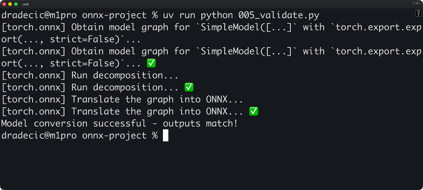

Veuillez exécuter cette validation à chaque fois que vous convertissez un modèle. De petites différences numériques sont normales (les calculs en virgule flottante ne sont pas exacts), mais des différences importantes indiquent qu'un problème est survenu lors de la conversion.

Pour conclure, voici deux mises en garde importantes dont vous devez tenir compte :

• Les opérations personnalisées ne seront pas converties : Si vous avez écrit des opérations PyTorch ou des couches TensorFlow personnalisées, le convertisseur ne saurait pas comment les traduire. Vous devez soit les réécrire à l'aide d'opérations standard, soit enregistrer des opérateurs ONNX personnalisés.
• Les incompatibilités de version peuvent entraîner des dysfonctionnements : La version de votre framework, la version du convertisseur et la version ONNX doivent être compatibles. Veuillez consulter la documentation du convertisseur pour connaître les combinaisons de versions prises en charge.

Ensuite, nous aborderons ONNX Runtime.

Exécution de l'inférence avec ONNX Runtime

Dans cette section, je vais vous expliquer comment utiliser ONNX Runtime pour charger des modèles et effectuer des prédictions. Je vais vous présenter les options d'accélération matérielle et vous montrer les domaines dans lesquels ONNX Runtime excelle en production.

Présentation d'ONNX Runtime

ONNX Runtime est un moteur d'inférence multiplateforme. Microsoft l'a développé pour exécuter rapidement les modèles ONNX sur n'importe quel matériel : processeurs, cartes graphiques, puces mobiles et accélérateurs IA spécialisés.

Voici comment cela fonctionne : Vous chargez un modèle ONNX, et ONNX Runtime élabore un plan d'exécution. Il analyse le graphe de calcul, applique des optimisations et détermine la meilleure façon d'exécuter les opérations sur votre matériel. Ensuite, il exécute l'inférence à l'aide du plan optimisé.

L'architecture sépare la logique d'exécution du code spécifique au matériel. Les fournisseurs d'exécution gèrent l'interface matérielle. Souhaitez-vous utiliser les GPU NVIDIA ? Veuillez utiliser le fournisseur d'exécution CUDA. Souhaitez-vous Apple Silicon ? Votre code sous-jacent reste inchangé.

ONNX Runtime dispose des fournisseurs d'exécution suivants :

• CPUExecutionProvider: Fournisseur par défaut, fonctionne partout

• CUDAExecutionProvider: Cartes graphiques NVIDIA avec CUDA

• TensorRTExecutionProvider: Cartes graphiques NVIDIA optimisées pour TensorRT

• CoreMLExecutionProvider: Appareils Apple (macOS, iOS)

• DmlExecutionProvider: DirectML pour Windows (compatible avec tous les GPU)

• OpenVINOExecutionProvider: Processeurs et processeurs graphiques Intel

• ROCMExecutionProvider: Processeurs graphiques AMD

Chaque fournisseur convertit les opérations ONNX en instructions spécifiques au matériel. Le fournisseur de CPU utilise des opérations CPU standard. Le fournisseur CUDA utilise cuDNN et cuBLAS. Le fournisseur TensorRT compile votre modèle en noyaux GPU optimisés, etc.

Mise en place et exécution d'un modèle

Vous pouvez charger un modèle ONNX à l'aide de trois lignes de code :

import onnxruntime as ort

# Create an inference session
session = ort.InferenceSession("simple_model.onnx")

# Get input and output names
input_name = session.get_inputs()[0].name
output_name = session.get_outputs()[0].name

L'InferenceSession e se charge de toutes les tâches complexes. Il charge le modèle, valide le graphe et se prépare pour l'inférence. Par défaut, il utilise le fournisseur d'exécution CPU.

Veuillez maintenant exécuter l'inférence :

import numpy as np
import onnxruntime as ort

# Create an inference session
session = ort.InferenceSession("simple_model.onnx")

# Get input and output names
input_name = session.get_inputs()[0].name
output_name = session.get_outputs()[0].name

# Prepare input data
input_data = np.random.randn(1, 10).astype(np.float32)

# Run inference
outputs = session.run(
    [output_name],
    {input_name: input_data},
)

# Get predictions
predictions = outputs[0]
print(predictions.shape)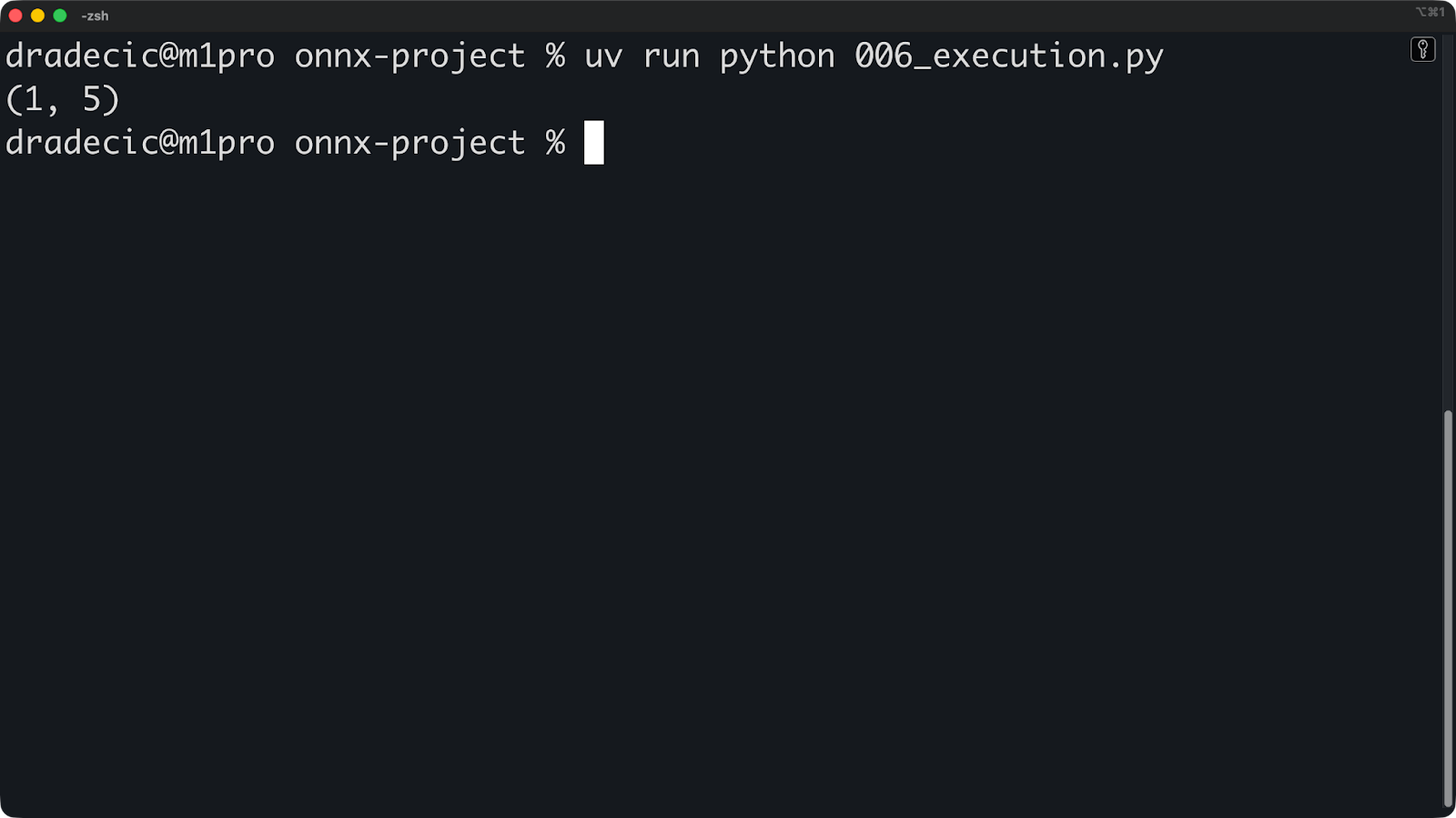

La méthode ` run() ` prend deux arguments. Tout d'abord, une liste des noms de sortie (ou l'None e pour toutes les sorties). Deuxièmement, un dictionnaire associant les noms d'entrée aux tableaux numpy.

Les formes d'entrée doivent correspondre. Si votre modèle attend [1, 10] et que vous transmettez [1, 10, 3], l'inférence échouera.

Si vous souhaitez bénéficier de l'accélération GPU, veuillez simplement spécifier les fournisseurs d'exécution lors de la création de la session :

# For NVIDIA GPUs with CUDA
session = ort.InferenceSession(
    "model.onnx",
    providers=['CUDAExecutionProvider', 'CPUExecutionProvider']
)

# For Apple Silicon
session = ort.InferenceSession(
    "model.onnx",
    providers=['CoreMLExecutionProvider', 'CPUExecutionProvider']
)

# For Intel hardware
session = ort.InferenceSession(
    "model.onnx",
    providers=['OpenVINOExecutionProvider', 'CPUExecutionProvider']
)

Veuillez énumérer les fournisseurs par ordre de priorité. ONNX Runtime tente d'abord le premier fournisseur et, s'il n'est pas disponible, passe au suivant. Veuillez toujours inclure CPUExecutionProvider comme dernier recours.

Vous pouvez vérifier quel fournisseur est actuellement utilisé :

import numpy as np
import onnxruntime as ort

# Create an inference session
session = ort.InferenceSession(
    "simple_model.onnx", providers=["CoreMLExecutionProvider", "CPUExecutionProvider"]
)

# Get input and output names
input_name = session.get_inputs()[0].name
output_name = session.get_outputs()[0].name

# Prepare input data
input_data = np.random.randn(1, 10).astype(np.float32)

# Run inference
outputs = session.run(
    [output_name],
    {input_name: input_data},
)

# Get predictions
predictions = outputs[0]
print(predictions.shape)
print("Providers:")
print(session.get_providers())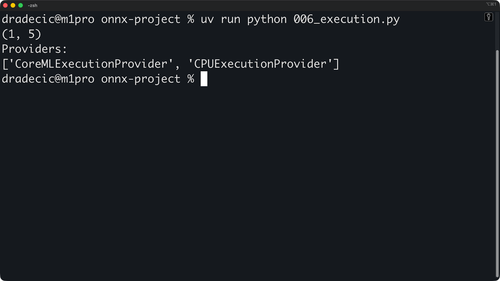

Si vous voyez « ["CPUExecutionProvider"] » alors que vous vous attendiez à un GPU, cela signifie que le fournisseur de GPU n'est pas disponible. Les raisons courantes peuvent être des pilotes manquants, un package ONNX Runtime incorrect ou un GPU incompatible.

La configuration ne s'arrête pas là. Vous pouvez optimiser davantage le fournisseur d'exécution afin d'obtenir de meilleures performances :

providers = [
    (
        "TensorRTExecutionProvider",
        {
            "device_id": 0,
            "trt_max_workspace_size": 2147483648,  # 2GB
            "trt_fp16_enable": True,  # Use FP16 precision
        },
    ),
    "CUDAExecutionProvider",
    "CPUExecutionProvider",
]

session = ort.InferenceSession("simple_model.onnx", providers=providers)

Veuillez consulter la documentation officielle d'ONNX Runtime pour obtenir la liste de toutes les options disponibles pour le fournisseur de votre choix.

Applications ONNX Runtime

Ce qui est remarquable avec ONNX Runtime, c'est qu'il fonctionne partout : sur les serveurs, les navigateurs et les appareils mobiles.

ONNX Runtime Web permet l'inférence dans les navigateurs à l'aide de WebAssembly et WebGL. Votre modèle fonctionne côté client sans envoyer de données aux serveurs. Ceci est particulièrement adapté aux applications sensibles en matière de confidentialité, telles que l'analyse d'images médicales ou le traitement de documents.

Voici un exemple illustrant comment utiliser ONNX Runtime dans un fichier HTML simple :

<!DOCTYPE html>
<html lang="en">
<head>
  <meta charset="UTF-8" />
  <meta name="viewport" content="width=device-width, initial-scale=1.0" />
  <title>ONNXRuntime Web Demo</title>
</head>
<body>
  <h1>ONNXRuntime Web Demo</h1>

  <!-- Load ONNXRuntime-Web from CDN -->
  <script src="<https://cdn.jsdelivr.net/npm/onnxruntime-web/dist/ort.min.js>"></script>

  <script>
    async function runModel() {
      // Create inference session
      const session = await ort.InferenceSession.create('./simple_model.onnx');

      // Prepare input
      const inputData = new Float32Array(10).fill(0).map(() => Math.random());
      const tensor = new ort.Tensor('float32', inputData, [1, 10]);

      // Run inference
      const results = await session.run({ input: tensor });

      const output = results.output;
      console.log('Output shape:', output.dims);
      console.log('Output values:', output.data);
    }

    runModel();
  </script>
</body>
</html>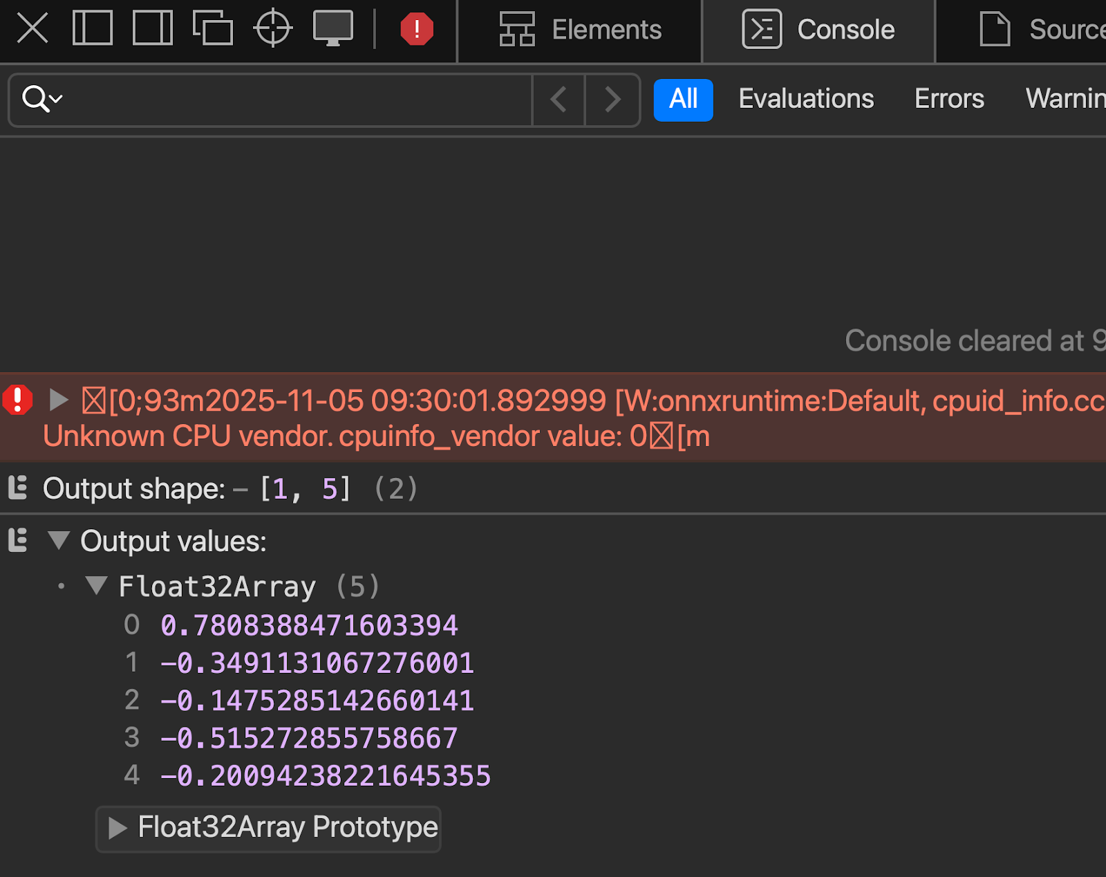

Pour un déploiement mobile, vous pouvez utiliser ONNX Runtime Mobile, une version allégée optimisée pour iOS et Android. Il supprime les fonctionnalités inutiles et réduit la taille du fichier binaire.

Voici un exemple de configuration iOS :

import onnxruntime_objc

let modelPath = Bundle.main.path(forResource: "simple_model", ofType: "onnx")!
let session = try ORTSession(modelPath: modelPath)

let inputData = // Your input as Data
let inputTensor = try ORTValue(tensorData: inputData,
                               elementType: .float,
                               shape: [1, 10])

let outputs = try session.run(withInputs: ["input": inputTensor])

Ou, si vous utilisez Python pour créer une API REST, vous pouvez inclure ONNX Runtime à l'un de vos points de terminaison en suivant cette approche :

from fastapi import FastAPI
import onnxruntime as ort
import numpy as np

app = FastAPI()
session = ort.InferenceSession("simple_model.onnx")

@app.post("/predict")
async def predict(data: dict):
    input_data = np.array(data["input"]).astype(np.float32)
    outputs = session.run(None, {"input": input_data})
    return {"prediction": outputs[0].tolist()}

Et voilà ! D'autres environnements utiliseront une approche similaire, mais vous comprenez l'essentiel : ONNX Runtime est facile à utiliser. Ensuite, nous aborderons l'optimisation.

Optimisation des modèles ONNX

Dans cette section, je vais vous montrer comment accélérer et réduire la taille des modèles ONNX grâce à la quantification et à l'optimisation des graphes. Je vais vous présenter les techniques les plus importantes pour les déploiements dans le monde réel.

Techniques de quantification

La quantification réduit la précision de votre modèle afin de le rendre plus rapide et plus compact.

Au lieu de stocker les poids sous forme de nombres flottants 32 bits, vous les stockez sous forme d'entiers 8 bits. Cela réduit l'utilisation de la mémoire de 75 % et accélère l'inférence, car les calculs mathématiques sur les nombres entiers sont plus rapides que ceux sur les nombres à virgule flottante sur la plupart des matériels.

La quantification dynamique convertit les poids en une précision inférieure, mais conserve les activations (valeurs intermédiaires pendant l'inférence) dans leur précision totale. Il s'agit de la méthode de quantification la plus simple, car elle ne nécessite pas de données d'étalonnage.

Voici comment appliquer la quantification dynamique :

from onnxruntime.quantization import quantize_dynamic, QuantType

# Quantize the model
quantize_dynamic(
    model_input="model.onnx",
    model_output="model_quantized.onnx",
    weight_type=QuantType.QUInt8  # 8-bit unsigned integers
)

C'est tout. Votre modèle quantifié utilise désormais des entiers non signés de 8 bits et est prêt à être utilisé.

La quantification statique convertit à la fois les poids et les activations en une précision inférieure. Elle est plus agressive et plus rapide que la quantification dynamique, mais il est nécessaire de disposer de données d'étalonnage représentatives pour mesurer les plages d'activation.

Voici une stratégie générale pour appliquer la quantification statique :

from onnxruntime.quantization import quantize_static, CalibrationDataReader
import numpy as np

# Create a calibration data reader
class DataReader(CalibrationDataReader):
    def __init__(self, calibration_data):
        self.data = calibration_data
        self.index = 0

    def get_next(self):
        if self.index >= len(self.data):
            return None
        batch = {"input": self.data[self.index]}
        self.index += 1
        return batch

# Load calibration data (100-1000 samples from your dataset)
calibration_data = [np.random.randn(1, 10).astype(np.float32)
                    for _ in range(100)]
data_reader = DataReader(calibration_data)

# Quantize
quantize_static(
    model_input="model.onnx",
    model_output="model_static_quantized.onnx",
    calibration_data_reader=data_reader
)

Les données d'étalonnage doivent refléter votre charge de travail d'inférence réelle. Par conséquent, veuillez éviter d'utiliser des données aléatoires comme celles présentées ci-dessus. Veuillez utiliser des échantillons réels provenant de votre ensemble de données.

En général, la quantification présente certains avantages et inconvénients qu'il est important de connaître en tant qu'ingénieur en apprentissage automatique. Voici les avantages :

• Modèles 4 fois plus petits : INT8 utilise un quart de la mémoire de FP32.
• Inference 2 à 4 fois plus rapide : Les opérations sur les nombres entiers s'exécutent plus rapidement sur les processeurs.
• Consommation d'énergie réduite : Moins de calculs signifie moins d'énergie
• Meilleure utilisation du cache : Les modèles plus petits s'adaptent au cache du processeur.

Et voici les compromis :

• Légère perte de précision : Généralement 1 à 2 % pour INT8, ce qui est acceptable pour la plupart des applications.
• Toutes les opérations ne se quantifient pas de manière optimale : La normalisation par lots et la fonction softmax peuvent être complexes.
• Dépendance matérielle : Les accélérations GPU varient, certains GPU n'accélèrent pas INT8.

La quantification est également très utile pour les grands modèles linguistiques et l'IA générative. Un modèle à 7 milliards de paramètres en FP32 nécessite 28 Go de mémoire. Une fois quantifié en INT8, il diminue à 7 Go. Quantifié en INT4, il occupe 3,5 Go, ce qui est suffisamment compact pour fonctionner sur du matériel grand public.

Optimisations graphiques

Les optimisations graphiques réécrivent le graphe de calcul de votre modèle afin d'accélérer son fonctionnement.

Le concept de fusion de nœuds regroupe plusieurs opérations en une seule opération. Si votre modèle comporte une couche Conv suivie d'une couche BatchNorm puis d'une couche ReLU, l'optimiseur les fusionne en un seul nœud d'ConvBnRelu. Cela réduit le trafic mémoire et accélère l'exécution.

Voici à quoi ressemble le graphique avant la fusion :

Input -> Conv -> BatchNorm -> ReLU -> Output

Après fusion, cela est simplifié :

Input -> ConvBnRelu -> Output

Il existe deux autres concepts que vous devez connaître en matière d'optimisation de graphes :

• Le pliage constant précalcule les opérations qui ne dépendent pas des données d'entrée. Si votre modèle multiplie une matrice de poids par une constante, l'optimiseur effectue cette multiplication une seule fois pendant l'optimisation, plutôt qu'à chaque inférence.
• L'élimination du code mort supprime les opérations inutilisées. Si votre modèle comporte des branches qui ne sont jamais exécutées ou des sorties que vous n'utilisez jamais, l'optimiseur les supprime.

Voici comment activer les optimisations graphiques dans ONNX Runtime :

import onnxruntime as ort

# Set optimization level
sess_options = ort.SessionOptions()
sess_options.graph_optimization_level = ort.GraphOptimizationLevel.ORT_ENABLE_ALL

# Create session with optimizations
session = ort.InferenceSession(
    "simple_model.onnx",
    sess_options,
    providers=["CPUExecutionProvider"]
)

ONNX Runtime propose les niveaux d'optimisation suivants :

• ORT_DISABLE_ALL: Aucune optimisation (utile pour le débogage)

• ORT_ENABLE_BASIC: Optimisations sécurisées qui ne modifient pas les résultats numériques

• ORT_ENABLE_EXTENDED: Les optimisations agressives peuvent entraîner de légères différences numériques.

• ORT_ENABLE_ALL: Toutes les optimisations, y compris les transformations de mise en page

Veuillez utiliser ORT_ENABLE_ALL pour la production. L'accélération justifie les différences numériques minimes.

Vous pouvez exécuter cet extrait de code pour enregistrer des modèles optimisés en vue d'une réutilisation :

sess_options = ort.SessionOptions()
sess_options.graph_optimization_level = ort.GraphOptimizationLevel.ORT_ENABLE_ALL
sess_options.optimized_model_filepath = "model_optimized.onnx"

# This creates and saves the optimized model
session = ort.InferenceSession("simple_model.onnx", sess_options)

Les optimisations graphiques fonctionnent quel que soit le framework utilisé pour créer votre modèle. Un modèle PyTorch Conv-BN-ReLU et un modèle TensorFlow Conv-BN-ReLU sont fusionnés de la même manière. C'est l'avantage de l'optimisation partagée : vous écrivez l'optimisation une seule fois, puis vous l'appliquez aux modèles de n'importe quel cadre.

Ensuite, nous aborderons le déploiement.

Scénarios de déploiement

Dans cette section, je vais aborder trois scénarios de déploiement : les périphériques, l'infrastructure cloud et les navigateurs web. Je vais vous présenter les défis et les solutions pour chaque environnement.

Déploiement de périphériques

Le principal défi des appareils périphériques réside dans leurs ressources limitées.

Votre smartphone dispose de 4 à 16 Go de mémoire vive. Un Raspberry Pi en a encore moins. Les appareils IoT peuvent disposer de 512 Mo ou moins. Il n'est pas possible de simplement appliquer un modèle à 7 milliards de paramètres à ces appareils et s'attendre à ce qu'il fonctionne.

Commencez par la quantification. Les modèles INT8 devraient constituer votre référence. Optez pour INT4 si vous pouvez accepter la perte de précision. Cela permet de réduire suffisamment la taille de votre modèle pour qu'il tienne dans la mémoire.

Pour le déploiement sur des appareils périphériques, ONNX Runtime Mobile est votre allié. Il supprime les fonctionnalités du serveur dont vous n'avez pas besoin et optimise l'autonomie de la batterie. Le fichier binaire est plus petit, le démarrage est plus rapide et la consommation d'énergie est réduite.

Voici comment l'intégrer à votre projet d'application mobile :

# iOS
pod 'onnxruntime-mobile-objc'

# Android
implementation 'com.microsoft.onnxruntime:onnxruntime-android:latest.version'

Les fournisseurs d'exécution gèrent les différences matérielles. Les appareils Android utilisent des processeurs ARM, certains sont équipés de processeurs graphiques provenant de différents fournisseurs, et les téléphones plus récents intègrent des processeurs neuronaux (NPU). Il n'est pas souhaitable d'écrire du code pour chaque puce.

Veuillez vous référer à cet extrait pour sélectionner le fournisseur d'exécution approprié :

# iOS - use CoreML for Apple Silicon optimization
session = ort.InferenceSession(
    "simple_model.onnx",
    providers=["CoreMLExecutionProvider", "CPUExecutionProvider"]
)

# Android - use NNAPI for hardware acceleration
session = ort.InferenceSession(
    "simple_model.onnx",
    providers=["NnapiExecutionProvider", "CPUExecutionProvider"]
)

CoreML sur iOS utilise le Neural Engine (NPU d'Apple). NNAPI sur Android utilise tous les accélérateurs disponibles sur votre appareil : GPU, DSP ou NPU. Le fournisseur abstrait le matériel afin que votre code reste inchangé. Lorsqu'une nouvelle puce offrant de meilleures performances est disponible, il suffit de mettre à jour le fournisseur d'exécution pour que votre application fonctionne plus rapidement sans modification du code.

Déploiement dans le cloud

Le déploiement dans le cloud vous offre une évolutivité illimitée et le matériel le plus récent.

Vous pouvez déployer des modèles ONNX sur n'importe quelle plateforme cloud : AWS, Azure, GCP ou vos propres serveurs. Le modèle est identique : conteneurisez votre service d'inférence et déployez-le derrière un équilibreur de charge.

Voici un exemple Python FastAPI succinct :

from fastapi import FastAPI, HTTPException
from pydantic import BaseModel
import onnxruntime as ort
import numpy as np
import logging

app = FastAPI()
logger = logging.getLogger(__name__)

# Load model at startup
session = None

@app.on_event("startup")
async def load_model():
    global session
    session = ort.InferenceSession(
        "simple_model.onnx",
        providers=[
            "CUDAExecutionProvider",
            "CoreMLExecutionProvider",
            "CPUExecutionProvider",
        ],
    )
    logger.info("Model loaded successfully")

class PredictionRequest(BaseModel):
    input: list

class PredictionResponse(BaseModel):
    prediction: list
    inference_time_ms: float

@app.post("/predict", response_model=PredictionResponse)
async def predict(request: PredictionRequest):
    try:
        import time

        start = time.time()

        # Input shape: (1, 10)
        input_data = np.array(request.input, dtype=np.float32).reshape(1, 10)
        input_name = session.get_inputs()[0].name
        outputs = session.run(None, {input_name: input_data})

        inference_time = (time.time() - start) * 1000

        return PredictionResponse(
            prediction=outputs[0].tolist(), inference_time_ms=inference_time
        )
    except Exception as e:
        logger.error(f"Prediction failed: {str(e)}")
        raise HTTPException(status_code=500, detail=str(e))

@app.get("/health")
async def health():
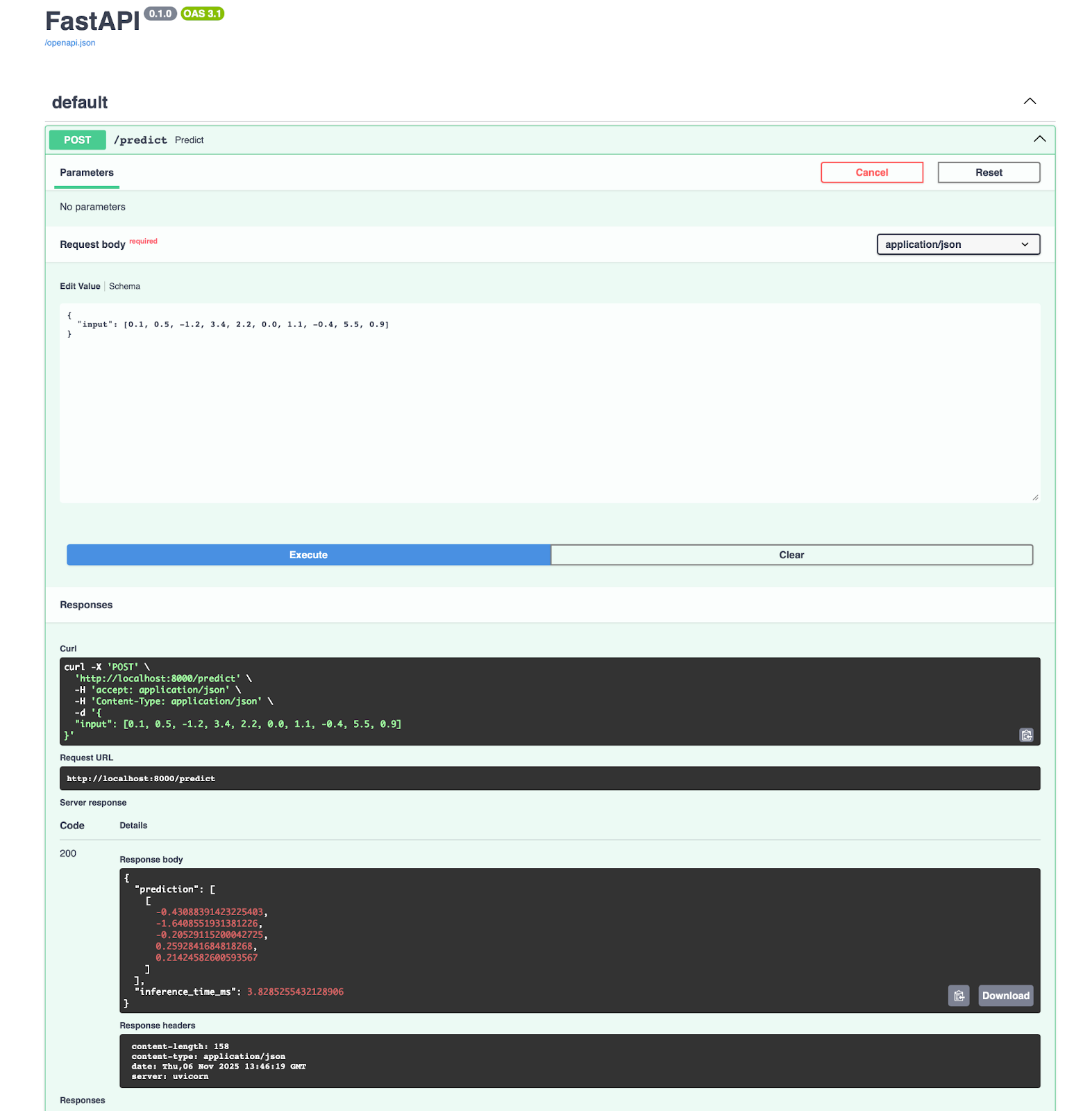
    return {"status": "healthy", "model_loaded": session is not None}

Cet exemple FastAPI, bien que succinct, n'est pas le plus facile à appréhender pour les ingénieurs en apprentissage automatique. Vous pouvez acquérir les bases grâce à notre cours gratuit cours d'introduction à FastAPI.

Vous pouvez ensuite le conteneuriser avec Docker :

FROM python:3.13-slim

WORKDIR /app

# Install dependencies
RUN pip install onnx onnxruntime onnxscript fastapi pydantic numpy uvicorn

# Copy model and code
COPY simple_model.onnx .
COPY main.py .

# Expose port
EXPOSE 8000

# Run the service
CMD ["uvicorn", "main:app", "--host", "0.0.0.0", "--port", "8000"]

Tout passionné d'apprentissage automatique doit connaître les bases de Docker. Veuillez consulter notre cours d'introduction à Docker pour enfin apprendre à déployer un modèle d'apprentissage automatique.

Vous obtiendrez une application fonctionnant sur le port 8000, pour laquelle vous pouvez ouvrir directement la documentation et tester le point de terminaison de prédiction :

Si vous utilisez Azure Machine Learning, vous serez heureux d'apprendre qu'il s'intègre directement à ONNX. Vous pouvez déployer votre modèle en trois étapes :

from azureml.core import Workspace, Model
from azureml.core.webservice import AciWebservice, Webservice

# Register model
ws = Workspace.from_config()
model = Model.register(
    workspace=ws, model_path="simple_model.onnx", model_name="my-onnx-model"
)

# Deploy
deployment_config = AciWebservice.deploy_configuration(cpu_cores=1, memory_gb=1)

service = Model.deploy(
    workspace=ws,
    name="onnx-service",
    models=[model],
    deployment_config=deployment_config,
)

Azure gère la mise à l'échelle, la surveillance et les mises à jour. Vous bénéficiez d'une journalisation automatique, d'un suivi des requêtes et de contrôles de santé.

Si vous débutez avec Azure Machine Learning, veuillez consulter notre Guide du débutant pour acquérir rapidement les connaissances de base.

Si nous parlons de workflows MLOps , les composants suivants sont nécessaires :

• s relatives au contrôle de version: Suivez le cursus des versions des modèles avec DVC ou MLflow
• S CI/CD: Automatisez les tests et le déploiement avec GitHub Actions ou Azure Pipelines.
• s de surveillance: Suivre la latence d'inférence, le débit et les taux d'erreur
• s sur les tests A/B: Veuillez comparer les versions des modèles en production.
• s de restauration: Revenir aux versions précédentes en cas de problèmes

Voici un exemple d'extrait que vous pouvez utiliser :

import prometheus_client as prom
import onnxruntime as ort
import numpy as np

# Define metrics
inference_duration = prom.Histogram(
    "model_inference_duration_seconds", "Time spent processing inference"
)

inference_count = prom.Counter("model_inference_total", "Total number of inferences")

# Load model
session = ort.InferenceSession("simple_model.onnx")

@app.post("/predict")
@inference_duration.time()
async def predict(request: PredictionRequest):
    inference_count.inc()
    # Input shape: (1, 10)
    input_data = np.array(request.input, dtype=np.float32).reshape(1, 10)
    input_name = session.get_inputs()[0].name
    outputs = session.run(None, {input_name: input_data})
    return {"prediction": outputs[0].tolist()}

À partir de là, vous pouvez procéder à une mise à l'échelle horizontale en exécutant plusieurs instances de service derrière un équilibreur de charge. ONNX Runtime est sans état, ce qui signifie que n'importe quelle instance peut traiter n'importe quelle requête.

Inférence basée sur le navigateur

ONNX Runtime Web exécute les modèles directement dans les navigateurs à l'aide de WebAssembly et WebGL.

Au lieu d'envoyer des données à un serveur, vous transmettez le modèle au navigateur une seule fois et effectuez l'inférence localement. Les utilisateurs obtiennent des réponses instantanées sans latence réseau.

Pour commencer, veuillez créer un fichier HTML qui utilise un script JS en ligne :

<!doctype html>
<html>
  <head>
    <meta charset="utf-8" />
    <script src="<https://cdn.jsdelivr.net/npm/onnxruntime-web/dist/ort.min.js>"></script>
  </head>
  <body>
    <script>
      async function run() {
        try {
          const session = await ort.InferenceSession.create("simple_model.onnx", {
            executionProviders: ["wasm"]
          });
          console.log("Session loaded:", session);

          // Inspect names
          console.log("Inputs:", session.inputNames);
          console.log("Outputs:", session.outputNames);

          const inputName = session.inputNames[0];

          const inputData = new Float32Array(10).fill(0).map(() => Math.random());
          const tensor = new ort.Tensor("float32", inputData, [1, 10]);

          const feeds = {};
          feeds[inputName] = tensor;

          const results = await session.run(feeds);

          const outputName = session.outputNames[0];
          console.log("Prediction:", results[outputName].data);

        } catch (err) {
          console.error("ERROR:", err);
        }
      }

      run();
    </script>
  </body>
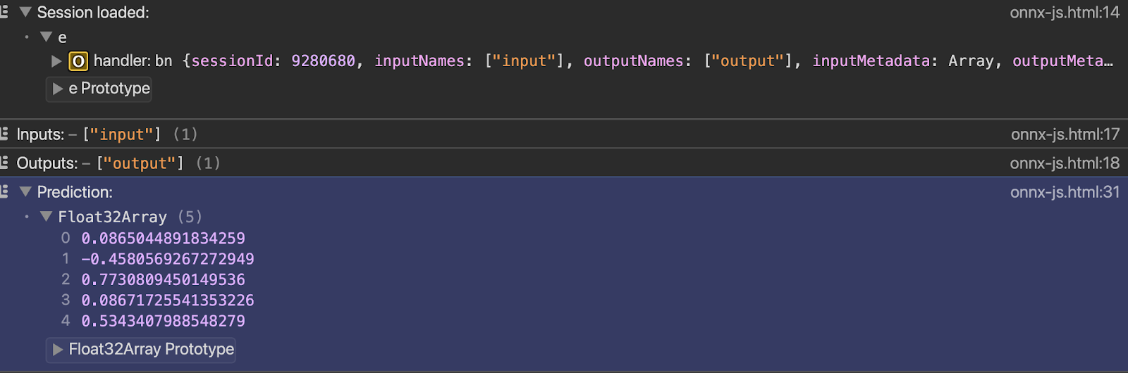
</html>

Vous pouvez observer le résultat dans la console dès que vous ouvrez le fichier avec le serveur en direct :

Enfin, abordons quelques sujets avancés.

Sujets avancés

Les opérations ONNX standard couvrent la plupart des cas d'utilisation, mais si vous avez besoin de plus, cette section est faite pour vous.

Je vais aborder les opérateurs personnalisés et le déploiement de grands modèles linguistiques. Je vous expliquerai quand vous aurez besoin de ces fonctionnalités avancées et quels compromis elles impliquent.

Opérateurs personnalisés

ONNX comprend des centaines d'opérations, mais il est possible que votre modèle utilise une opération spécifique.

Les opérateurs personnalisés vous permettent de définir des opérations qui ne sont pas disponibles dans l'ensemble d'opérateurs ONNX standard. Vous rédigez vous-même la logique opérationnelle et indiquez à ONNX Runtime comment l'exécuter. Cela étend les capacités intégrées d'ONNX.

Quand avez-vous besoin d'opérateurs personnalisés ? Lorsque vous utilisez des recherches de pointe qui ne sont pas encore prises en charge par ONNX. Ou lorsque vous avez mis en place des opérations propriétaires spécifiques à votre domaine. Ou lorsque vous avez besoin d'optimisations spécifiques au matériel que les opérations standard ne peuvent pas fournir.

Cependant, il y a un inconvénient : les opérateurs personnalisés compromettent la portabilité.. Votre modèle ne fonctionnera pas sur les systèmes qui ne disposent pas de votre implémentation d'opérateur personnalisée. Si vous exportez un modèle PyTorch avec des opérations personnalisées vers ONNX, il est nécessaire de regrouper ces opérations séparément et de les enregistrer avec ONNX Runtime.

Le déploiement devient plus complexe. Chaque environnement nécessite votre bibliothèque d'opérateurs personnalisée. Les périphériques, les serveurs cloud et les navigateurs nécessitent tous la même implémentation. Vous perdez le principal avantage d'ONNX : écrire une fois, exécuter partout.

Voici un petit exemple fonctionnel d'opérateurs personnalisés, afin que vous puissiez observer leur fonctionnement :

import numpy as np
import onnxruntime as ort
from onnxruntime import InferenceSession, SessionOptions

# Define the custom operation
def custom_square(x):
    return x * x

# Register the custom op with ONNX Runtime
# This tells ONNX Runtime how to execute "CustomSquare" operations
class CustomSquareOp:
    @staticmethod
    def forward(x):
        return np.square(x).astype(np.float32)

# Create a simple ONNX model with a custom op using the helper
from onnx import helper, TensorProto
import onnx

# Create a graph with custom operator
node = helper.make_node(
    "CustomSquare",  # Custom operation name
    ["input"],
    ["output"],
    domain="custom.ops",  # Custom domain
)

graph = helper.make_graph(
    [node],
    "custom_op_model",
    [helper.make_tensor_value_info("input", TensorProto.FLOAT, [1, 10])],
    [helper.make_tensor_value_info("output", TensorProto.FLOAT, [1, 10])],
)

model = helper.make_model(graph)
onnx.save(model, "custom_op_model.onnx")

# To use this model, you'd need to implement the custom op in C++
# and register it with ONNX Runtime - Python-only custom ops aren't supported
print("Custom operator model created - requires C++ implementation to run")

La plupart des équipes évitent les opérateurs personnalisés lorsque cela est possible. Veuillez d'abord essayer d'utiliser des combinaisons d'opérations standard. Optez pour une solution personnalisée uniquement lorsque les opérations standard ne permettent pas de répondre à vos besoins opérationnels ou lorsque les performances l'exigent.

Gestion de modèles linguistiques de grande envergure

La mémoire représente un défi pour les modèles d'apprentissage profond. Un modèle à 7 milliards de paramètres nécessite 28 Go en FP32, 14 Go en FP16 et 7 Go en INT8. La plupart des équipements grand public ne sont pas en mesure de prendre en charge cela. Il est nécessaire de procéder à une quantification, souvent de manière significative, vers INT4 ou INT3.

Si vous débutez dans le domaine des LLM et souhaitez en savoir plus, notre cours sur les concepts des cours sur les concepts des grands modèles linguistiques (LLM) est un excellent point de départ.

La gestion de la mémoire cache KV est importante pour l' e de génération autorégressive. Chaque jeton que vous générez doit faire référence à tous les jetons précédents. La taille du cache augmente avec la longueur de la séquence. Les conversations prolongées consomment rapidement la mémoire. ONNX Runtime GenAI comprend une gestion optimisée du cache KV qui réutilise la mémoire et réduit la charge.

La vitesse d'inférence dépend de votre matériel et de la taille du modèle. Les modèles plus petits (moins de 3B paramètres) fonctionnent efficacement sur les processeurs graphiques grand public. Les modèles plus volumineux nécessitent plusieurs processeurs graphiques ou des accélérateurs d'inférence spécialisés. ONNX Runtime prend en charge l'inférence multi-GPU via des fournisseurs d'exécution, mais il est nécessaire de répartir manuellement votre modèle entre les différents appareils.

s de Flash Attention accélère le mécanisme d'attention dans les transformateurs. L'attention standard est de O(n²) en longueur de séquence - elle ralentit rapidement. Flash Attention réduit les mouvements de mémoire et améliore la vitesse sans modifier les résultats. ONNX Runtime comprend des optimisations Flash Attention pour le matériel pris en charge.

Il est possible de former des LLM avec ONNX Runtime, mais cela est peu courant. La plupart des équipes s'entraînent avec PyTorch ou JAX, puis exportent vers ONNX uniquement pour l'inférence. La formation ONNX Runtime est destinée au réglage fin et à la préformation continue, mais l'écosystème autour de la formation PyTorch est plus mature.

Les charges de travail d'IA générative bénéficient d'un traitement spécial dans ONNX Runtime. Les extensions GenAI fournissent des API de haut niveau pour la génération de texte, le maintien de l'état entre les appels et la gestion des stratégies de recherche par faisceau ou d'échantillonnage. Cela vous évite d'avoir à implémenter vous-même la logique de génération.

Le paysage LLM évolue rapidement, et les mises à jour d'ONNX Runtime s'efforcent de suivre le rythme. L'ensemble des opérateurs et les optimisations sont régulièrement mis à jour, mais il existe toujours un décalage entre la recherche et la prise en charge prête pour la production.

Conclusion

Vous savez désormais comment convertir des modèles à partir de n'importe quel framework, les optimiser pour la production et les déployer n'importe où.

ONNX élimine les obstacles entre la formation et le déploiement. Veuillez vous former à PyTorch, car il est particulièrement adapté à la recherche. Déployez avec ONNX Runtime, car il est rapide et fonctionne partout. Quantifiez en INT8 et réduisez de moitié vos coûts d'inférence. Passer du CPU au GPU sans modifier le code. Transférez vos modèles entre différents fournisseurs de services cloud sans dépendre d'un seul fournisseur.

C'est ONNX qui rend cela possible.

L'écosystème continue de s'améliorer. Le support de l'IA générative s'améliore à chaque nouvelle version : inférence LLM plus rapide, meilleure gestion de la mémoire et nouvelles techniques d'optimisation. La prise en charge matérielle s'étend à davantage d'accélérateurs et de périphériques de pointe. La communauté développe des outils qui facilitent l'utilisation d'ONNX. Vous pouvez participer en testant de nouvelles fonctionnalités, en signalant des problèmes ou en contribuant au code via les GitHub.

Êtes-vous prêt à passer au niveau supérieur ? Maîtrise Concepts d'intelligence artificielle explicable (XAI) pour enfin cesser de considérer les modèles comme des boîtes noires.