Twee kolommen vergelijken in Excel: een stapsgewijze gids

Twee kolommen vergelijken in Excel op overeenkomsten

Als je met data werkt, moet je vaak twee kolommen vergelijken om overeenkomsten te vinden. Excel biedt hiervoor verschillende methoden, elk met voordelen afhankelijk van de complexiteit van je gegevens.

Twee kolommen vergelijken met de gelijk-operator

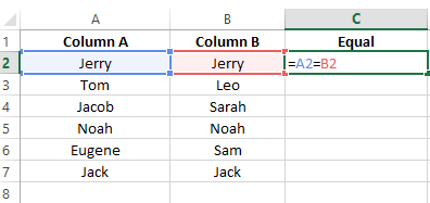
Een directe manier om twee kolommen in Excel te vergelijken is de gelijk-=-operator. De gelijk-operator controleert direct of de waarden in twee cellen hetzelfde zijn. Ik heb hier bijvoorbeeld twee kolommen—Kolom A en Kolom B. Ik heb ook een derde kolom toegevoegd en de volgende formule ingevoerd om te controleren of beide waarden gelijk zijn.

=A2=B2

Voer de gelijkheidsformule in een cel in. Afbeelding door auteur.

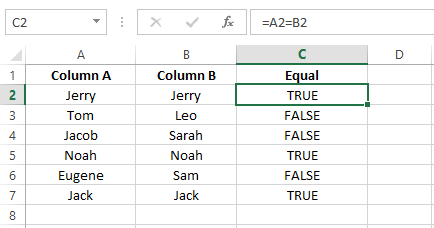
De =-operator vergelijkt de inhoud van twee cellen en retourneert TRUE als ze identiek zijn en FALSE als dat niet zo is. 

Controleren of twee kolommen gelijk zijn. Afbeelding door auteur.

Je kunt deze methode gebruiken wanneer je snel en eenvoudig gegevens in twee verschillende kolommen wilt vergelijken en wilt verifiëren of de invoer overeenkomt, bijvoorbeeld bij het vergelijken van lijsten met namen of productcodes.

Twee kolommen vergelijken met de IF()-functie

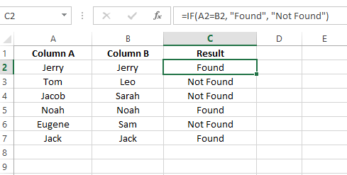
Omdat de =-operator alleen standaard TRUE of FALSE geeft, is het niet altijd ideaal, bijvoorbeeld als je een aangepaste uitvoer nodig hebt. In dat geval kun je de IF()-functie gebruiken. Hier is hetzelfde voorbeeld, maar nu gebruik ik een IF()-functie: 

=IF(A2=B2, "Found", "Not Found")

Voer de IF()-formule in de cel in. Afbeelding door auteur.

Ik heb de uitvoer aangepast naar mijn voorkeur. Ik schreef Found en Not Found, maar ik had hier eender wat kunnen zetten.

Pas het bericht aan met de IF()-functie. Afbeelding door auteur.

Twee kolommen vergelijken met de EXACT()-functie

De EXACT()-functie vergelijkt twee waarden met een hoofdlettergevoelige vergelijking, wat handig is wanneer je onderscheid moet maken tussen hoofd- en kleine letters. Ik heb bijvoorbeeld twee kolommen, Kolom A en Kolom B, en een derde kolom genaamd Resultaat, waar ik de volgende formule invoer:

=EXACT(A2,B2)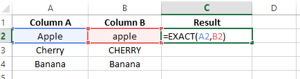

Voer de EXACT()-formule in een cel in. Afbeelding door auteur.

Je ziet dat ik Apple en Cherry met twee verschillende hoofdlettergebruik heb geschreven, en wanneer ik de formule toepas, wordt FALSE weergegeven, ook al zijn de namen hetzelfde. Dat komt doordat het een hoofdlettergevoelige formule is, die onderscheid maakt tussen hoofd- en kleine letters.

 Vergelijk hoofdlettergevoelige waarden met de Exact()-functie. Afbeelding door auteur.

Wil je de waarden TRUE of FALSE vervangen door je eigen bericht, omkader je formule dan met de IF()-functie zoals ik hieronder heb gedaan.

=IF(EXACT(A2,B2),"Match","Mismatch")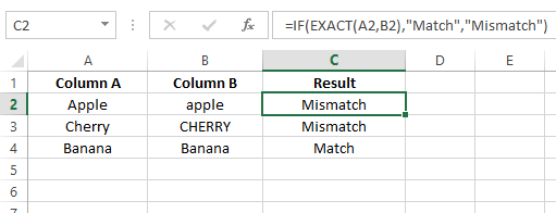

Combineer IF() met EXACT() om het bericht aan te passen. Afbeelding door auteur.

Deze methode is ideaal voor het verifiëren van gebruikersnamen, productcodes of andere tekststrings waarbij het verschil tussen hoofd- en kleine letters tot andere uitkomsten kan leiden.

Twee kolommen vergelijken met voorwaardelijke opmaak

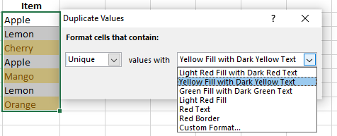
Voorwaardelijke opmaak is een Excel-functie waarmee je verschillende opmaakstijlen op cellen kunt toepassen op basis van specifieke criteria. Om dubbele waarden in een kolom te markeren, volg je deze stappen:

• Selecteer het celbereik waarin je dubbele invoer wilt identificeren. 
• Ga vervolgens naar Start > Stijlen > Voorwaardelijke opmaak > Regels voor markeren van cellen > Dubbele waarden.

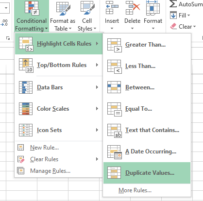
De optie voor dubbele waarden selecteren. Afbeelding door auteur

• Zodra het dialoogvenster verschijnt, zie je de lichtrode opvulling met donkerrood vooraf geselecteerde opmaak. Klik op OK. 

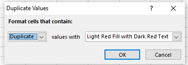
Illustratie van het dialoogvenster met dubbele waarden. Afbeelding door auteur.

Let op: Als je een andere opmaak verkiest, kun je in het vervolgkeuzemenu uit verschillende voorinstellingen kiezen. En als je een volledig andere weergave wilt, selecteer dan Aangepaste opmaak... onderaan het menu en kies je gewenste opvul- en letterkleuren. Klik op OK zodra je klaar bent. 

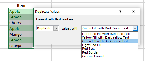
Markeer dubbele waarden met Voorwaardelijke opmaak. Afbeelding door auteur.

• Kies op dezelfde manier Uniek in het vervolgkeuzemenu om unieke waarden te markeren in plaats van Dubbel.

Markeer de unieke waarden. Afbeelding door auteur.

Voor een diepere duik in visuele markeringstechnieken, zie onze gids over duplicaten markeren in Excel, met extra regels voor voorwaardelijke opmaak en Power Query-aanpakken voor grote datasets.

Twee kolommen vergelijken met de VLOOKUP()-functie

Je kunt ook de VLOOKUP()-functie gebruiken om kolommen in Excel te vergelijken. Ik heb bijvoorbeeld dezelfde dataset als in het voorbeeld met de IF()-functie, maar hier heb ik de volgende formule ingevoerd:

=VLOOKUP(A2, $B$2:$B$10, 1, FALSE)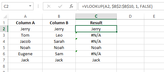

Gebruik VLOOKUP() om de waarden te vergelijken. Afbeelding door auteur.

Als je vergelijking fouten oplevert zoals in de bovenstaande afbeelding, plaats je formule dan binnen de IFERROR()-functie om dit af te handelen.

=IFERROR(VLOOKUP(A2, $B$2:$B$10, 1, FALSE), "Not Matched")

Zo werkt het:

• Er wordt gezocht naar de waarde in cel A2 binnen het bereik $B$2:$B10.

• Als er een exacte overeenkomst is gevonden, retourneert VLOOKUP() de overeenkomende waarde. 

• Als er geen overeenkomst is, retourneert IFERROR() Not Matched in plaats van de fout. 

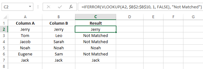
Fouten afhandelen met IFERROR() in combinatie met VLOOKUP(). Afbeelding door auteur.

Twee kolommen vergelijken met XLOOKUP() (Excel 365)

Als je Excel 365 of Excel 2021 gebruikt, biedt XLOOKUP() een flexibel alternatief voor VLOOKUP() bij kolomvergelijkingen. In tegenstelling tot VLOOKUP() zoekt het in elke richting, is geen kolomindexnummer nodig en verwerkt het ontbrekende waarden met een ingebouwde fallback—waardoor omwikkelen met IFERROR() niet nodig is.

=XLOOKUP(A2, $B$2:$B$10, $B$2:$B$10, "Not Found")

Zo werken de argumenten:

• A2 — de zoekwaarde (het item uit Kolom A dat je in Kolom B wilt vinden)
• $B$2:$B$10 (eerste instantie) — de zoekmatrix (waar te zoeken)
• $B$2:$B$10 (tweede instantie) — de resultaatmatrix (wat te retourneren bij een vondst)
• "Not Found" — de waarde die wordt geretourneerd als er geen overeenkomst is (vervangt IFERROR())

Dit retourneert de overeenkomende waarde uit Kolom B als die wordt gevonden, of “Not Found” als er geen match is. Voor gebruikers van Excel 2019 of eerder gebruik je de VLOOKUP()-aanpak hierboven. Wil je weten wanneer je welke kiest, bekijk dan onze XLOOKUP vs. VLOOKUP-vergelijkingsgids.

Twee kolommen vergelijken met matrixformules

Matrixformules kunnen meerdere waarden tegelijk verwerken. In plaats van met één waarde te werken, verwerken ze een gegevensbereik, waardoor complexe berekeningen efficiënter worden. Om een matrixformule te gebruiken, typ je deze in de cel en druk je op Ctrl+Shift+Enter.

Ik heb hier bijvoorbeeld twee kolommen—Kolom A en Kolom B. Nu wil ik bepalen of er een overeenkomst is tussen deze twee.

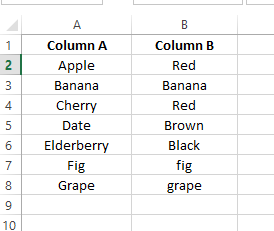
Kolom A en Kolom B bevatten data. Afbeelding door auteur.

Hiervoor gebruik ik de volgende formule: 

=SUM(--(A2=B2))

Hierbij geldt:

• De SUM()-functie telt de waarden in de array op. Als er minimaal één overeenkomst is, is de som groter dan 0. Anders is deze 0.
• De dubbele unair-operator (-- ) zet de TRUE- en FALSE-waarden om naar 1 en 0, wat resulteert in een array van 1'en en 0'en.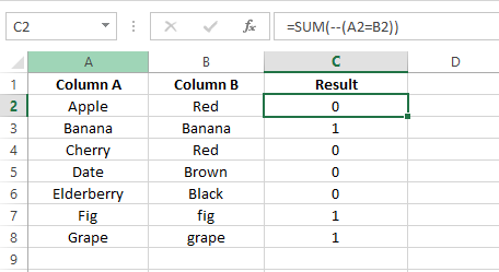

Kolommen vergelijken met SUM()-formules. Afbeelding door auteur.

Nu wil ik een aangepast bericht weergeven in plaats van 0'en en 1'en, dus plaats ik de SUM()-functie binnen een IF()-functie.

=IF(SUM(--(A2=B2))=0, "No match", "Match")

De IF()-functie controleert of de som 0 is. Als dat zo is, retourneert het No match. Anders retourneert het Match.

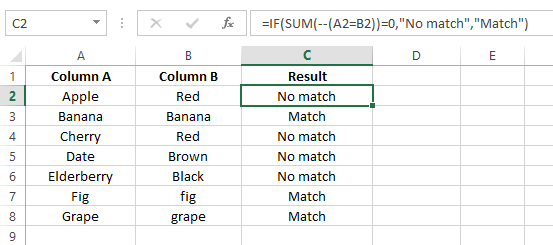
SUM()-formule binnen IF(). Afbeelding door auteur.

En klaar. Met de matrixformule kun je efficiënt vergelijkbare complexe vergelijkingen uitvoeren.

Twee kolommen vergelijken in Excel op duplicaten

Je weet nu hoe je kolommen op overeenkomsten vergelijkt, maar er zijn ook situaties waarin je duplicaten moet identificeren. Ter verduidelijking: overeenkomsten verwijzen naar corresponderende waarden in verschillende kolommen maar op dezelfde rij. Daarentegen verwijzen duplicaten specifiek naar waarden die één of meer keer voorkomen in beide kolommen maar op verschillende rijen. 

Twee kolommen vergelijken met IF() en MATCH()

De IF()- of MATCH()-functie alleen kan geen zoekopdrachten uitvoeren om duplicaten te identificeren. Maar als we ze samen gebruiken, kunnen we duplicaten vinden. Ik heb bijvoorbeeld een dataset met maandnamen in Kolom A en Kolom B. Vervolgens maak ik een extra kolom om de resultaten op te halen. Ik typ de volgende MATCH()-formule in de eerste cel en sleep deze naar de laatste cel om de dubbele waarden in mijn gegevensbereik te controleren.

=MATCH(A2,$B$2:$B$7,0)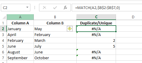

Duplicaten vinden met MATCH(). Afbeelding door auteur.

Je ziet echter dat als de waarde een duplicaat is—MATCH() de positie van de waarde uit de tweede kolom teruggeeft. Anders krijg je een #N/A-fout. In plaats van een #N/A-fout weer te geven, plaats je formule binnen de ISERROR()-functie. Deze geeft TRUE weer als er een #N/A-fout is. Anders FALSE.

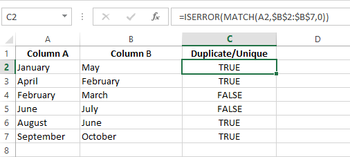
Fouten afhandelen met ISERROR(). Afbeelding door auteur.

Ik geef de voorkeur aan een aangepaste uitvoer in plaats van TRUE of FALSE. Voor een aangepaste uitvoer plaats je de formule binnen een IF()-functie zoals dit:

=IF(ISERROR(MATCH(A2,$B$2:$B$7,0)),"Unique","Duplicate")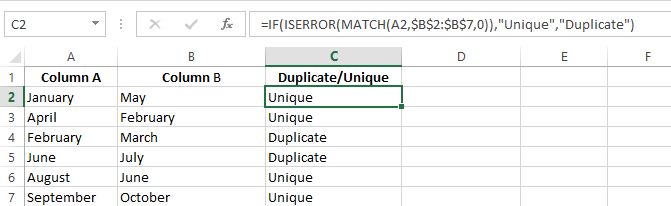

Duplicaten weergeven met de functies IF() en MATCH(). Afbeelding door auteur.

Twee kolommen vergelijken met COUNTIF()

Je kunt ook de COUNTIF()-functie gebruiken om twee kolommen te vergelijken en duplicaten te identificeren. Deze telt hoe vaak een waarde in de tweede kolom voorkomt en geeft 0 weer als de waarde uniek is en 1 als deze een duplicaat is. Bekijk de volgende formule:

=COUNTIF($B$2:$B$7,$A2:$A7)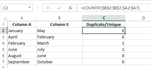

COUNTIF() gebruiken om dubbele waarden te controleren. Afbeelding door auteur.

Wil je een aangepast bericht weergeven in plaats van 0'en en 1, plaats de COUNTIF() dan in de IF()-functie.

=IF(COUNTIF($B$2:$B$7,$A2:$A7)=0,"Unique","Duplicate")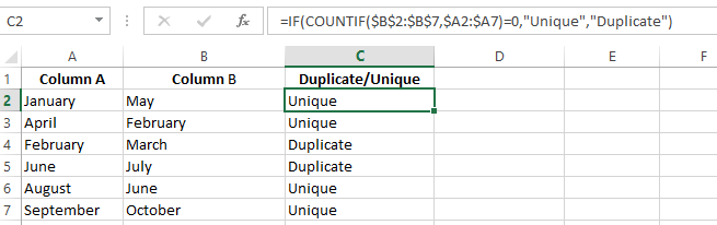

IF() gebruiken om aangepaste berichten weer te geven. Afbeelding door auteur.

De juiste vergelijkingsmethode kiezen

Met verschillende methoden beschikbaar, vind je hier een kort overzicht om je te helpen de juiste aanpak voor jouw situatie te kiezen:

Tot slot

Je zou nu een goed beeld moeten hebben van de verschillende methoden om twee kolommen in Excel te vergelijken, van de basis met de =-operator tot meer geavanceerde technieken zoals VLOOKUP() en matrixformules. Elke methode heeft zijn waarde, of je nu snelle vergelijkingen nodig hebt of complexere datavalidatie uitvoert. De verschillende methoden werken ook als je twee kolommen wilt vergelijken op overeenkomsten of op duplicaten.

Wil je je skills verder aanscherpen, bekijk dan ook andere bronnen. Begin met een cursus Inleiding tot Excel om een sterke basis te leggen. Ga daarna verder met de cursus Data-analyse in Excel om te leren hoe je ruwe data omzet in inzichtelijke rapporten.

Om je vaardigheden te boosten, overweeg het voltooien van de skill track Excel Fundamentals, die een breed scala aan essentiële functies en features behandelt. En vergeet niet de Excel Formulas Cheat Sheet te downloaden—een handige referentie voor binnen handbereik.