How to Compare Two Columns in Excel: A Step-by-Step Guide

How to Compare Two Columns in Excel for Matches

When working with data, you often need to compare two columns to identify matches. To do so, Excel offers several methods, each with advantages depending on the complexity of the data you have at hand.

Comparing two columns using the equals operator

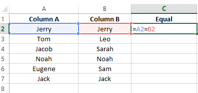
The easiest way to compare two columns in Excel is to use the equals = operator. The equals operator directly checks whether the values in two cells are the same. For example, I have two columns here—Column A and Column B. I also added a third column and entered the following formula to check whether both values are the same.

=A2=B2

Enter the Equal formula in a cell. Image by Author.

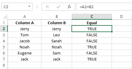
The = operator compares the content of two cells and returns TRUE if they are identical and FALSE if they are not. 

Checking if two columns are equal. Image by Author.

You can use this method when you need a quick and simple way to compare data in two different columns and verify whether their data entries match, such as when comparing lists of names or product codes.

Comparing two columns using the IF() function

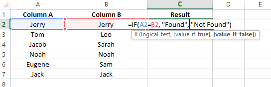
Since the = operator only gives default TRUE or FALSE, it’s not the ideal case for every need, such as when you need to create a custom output. If you need a custom output, you can use the IF() function instead. Here is the same example except this time I use an IF() function: 

=IF(A2=B2, "Found", "Not Found")

Enter the IF() formula in the cell. Image by Author.

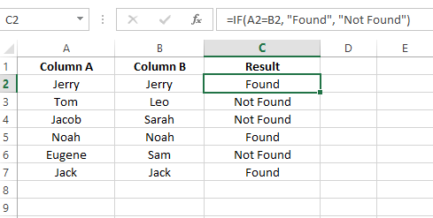
I customized the output according to my preference. I wrote Found and Not Found but I could have written anything.

Customize the message using the IF() function. Image by Author.

Comparing two columns using the EXACT() function

The EXACT() function compares two values by performing a case-sensitive comparison, which is helpful when you have to distinguish between uppercase and lowercase letters. For example, I have two columns, Column A and Column B, and a third column called Result, where I enter the following formula:

=EXACT(A2,B2)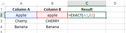

Enter the EXACT() formula in a cell. Image by Author.

You can see I’ve written Apple and Cherry with two different cases, and when I apply the formula, it displays FALSE even though the names are the same. The reason is that it’s a case-sensitive formula, so it distinguishes between uppercase and lowercase letters.

 Compare the case-sensitive values with the Exact() function. Image by Author.

If you want to replace the values TRUE or FALSE with your custom message, wrap your formula around the IF() function as I did below.

=IF(EXACT(A2,B2),"Match","Mismatch")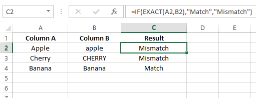

To customize the message, combine IF() with EXACT(). Image by Author.

This method is ideal when verifying usernames, product codes, or other text strings where the difference between uppercase and lowercase letters can lead to different outcomes.

Comparing two columns using conditional formatting

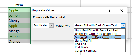
Conditional formatting is an Excel feature that allows you to apply different formatting styles to cells based on specific criteria. To highlight the duplicate values in a column, follow these steps:

• Select the range of cells where you'd like to identify duplicate entries. 
• Next, go to Home > Styles > Conditional Formatting > Highlight Cells Rules > Duplicate Values.

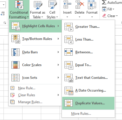
Selecting the duplicate values option. Image by Author

• Once the dialog box appears, you’ll see the light red filled with dark red format preselected. Hit OK. 

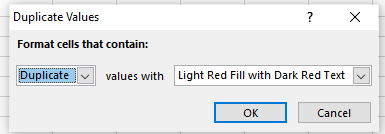
Illustration of the dialog box with duplicate values. Image by Author.

Note: If you prefer a different format, you can choose from several other pre-set formats in the dropdown menu. And if you want a completely different appearance, select Custom Format... at the bottom of the dropdown and pick your desired fill and font colors. Hit OK once you’re done. 

Highlight the duplicate values using Conditional Formatting. Image by Author.

• Similarly, select Unique from a drop-down menu to highlight the unique values instead of Duplicate.

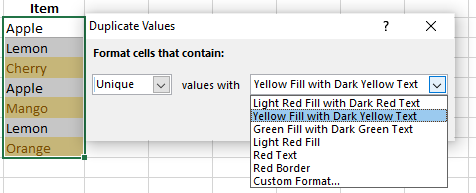
Highlight the unique values. Image by Author.

Comparing two columns with the VLOOKUP() function

You can also use the VLOOKUP() function to compare columns in Excel. For example, I have the same dataset from the IF() function example, but here, I entered the following formula:

=VLOOKUP(A2, $B$2:$B$10, 1, FALSE)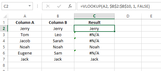

Use VLOOKUP() to compare the values. Image by Author.

If your comparison shows errors as shown in the above image, wrap your formula inside the IFERROR() function to handle it.

=IFERROR(VLOOKUP(A2, $B$2:$B$10, 1, FALSE), "Not Matched")

Here's how it works:

• It searches for the value in cell A2 within the range $B$2:$B10.

• If an exact match is found, VLOOKUP() returns the matched value. 

• If no match is found, IFERROR() then returns Not Matched instead of the error. 

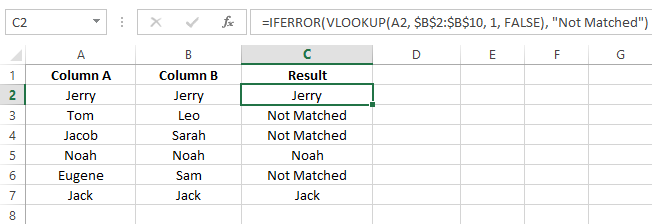
Handle the error using IFERROR() with VLOOKUP() function. Image by Author.

Comparing two columns using array formulas

Array formulas can handle multiple values at once. Instead of working on a single value, they process a range of data, making complex calculations more efficient. To use an array formula, type it in the cell and press Ctrl+Shift+Enter.

For example, I have two columns here—Column A and Column B. Now, I want to determine if there is a match between these two.

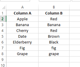
Column A and Column B contain data. Image by Author.

For this purpose, I’ll use the following formula: 

=SUM(--(A2=B2))

Here:

• The SUM() function adds up the values in the array. If there is at least one match, the sum will be greater than 0. Otherwise, it will be 0.
• The double unary operator (-- )converts the TRUE and FALSE values to 1 and 0, resulting in an array of 1s and 0s.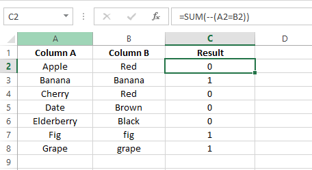

Comparing columns with SUM() formulas. Image by Author.

Now, I want to display a custom message instead of 0s and 1s, so I wrap the SUM() function inside an IF() function.

=IF(SUM(--(A2=B2))=0, "No match", "Match")

The IF() function checks if the sum is 0. If it is, it returns No match. Otherwise, it returns Match.

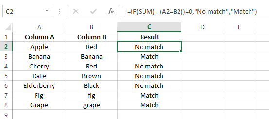
SUM() formula inside IF(). Image by Author.

And it's done. With the array formula, you can efficiently perform similar complex comparisons.

How to Compare Two Columns in Excel for Duplicates

You now know how to compare columns for the matches, but there are situations when you have to identify duplicates, too. To be clear, matches refer to corresponding values in different columns but in the same row. On the other hand, duplicates specifically refer to values that appear once or more across both columns but in different rows. 

Comparing two columns using IF() and MATCH()

The IF() function or the MATCH() function alone can’t perform lookups to identify duplicates. But if we use them together we can identify duplicates. For example, I have a dataset of month names organized in Column A and Column B. I then create another column to fetch the results. I type the following MATCH() formula in the first cell and dragged it to the last cell to check the duplicate values in my data range.

MATCH(A2,$B$2:$B$7,0)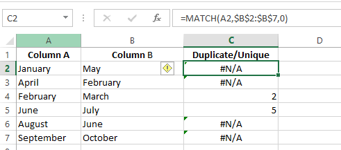

Using MATCH() to find duplicates. Image by Author.

But you can see if the value is duplicate—MATCH() returns the position of the value from the second column. Otherwise, it throws an #N/A error. Instead of displaying a #N/A error, wrap your formula inside the ISERROR() function. This will display TRUE if there is an #N/A error. Otherwise FALSE.

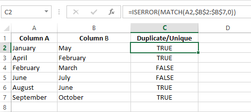
Handling errors using ISERROR(). Image by Author.

I prefer a custom output instead of TRUE or FALSE. For a custom output, wrap the formula inside an IF() function like this:

=IF(ISERROR(MATCH(A2,$B$2:$B$7,0)),"Unique","Duplicate")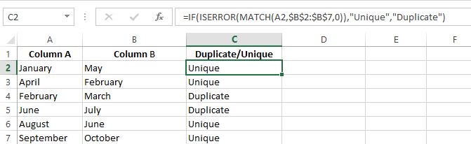

Displaying duplicate values using IF() and MATCH() functions. Image by Author.

Comparing two columns using COUNTIF()

You can also use the COUNTIF() function to compare two columns and identify duplicates. It identifies the occurrences of a value in the second column and displays 0 when the value is unique and 1 when it is a duplicate. Take a look at the following formula:

=COUNTIF($B$2:$B$7,$A2:$A7)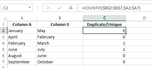

Using COUNTIF() to check the duplicate values. Image by Author.

If you want to display a custom message instead of 0s and 1, wrap the COUNTIF() inside the IF() function.

=IF(COUNTIF($B$2:$B$7,$A2:$A7)=0,"Unique","Duplicate")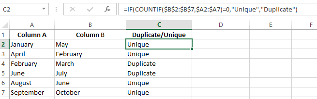

Using IF() to display the custom messages. Image by Author.

Final Thoughts

By now, you should have a solid understanding of the different methods you can use to compare two columns in Excel, from the primary = operator to more advanced techniques like VLOOKUP(), and array formulas. Each method has its value, whether you need quick comparisons or you are performing more complex data validation tasks. The different methods also work if you need to compare two columns for matches or for duplicates.

If you want to further sharpen your skills, I’d also encourage you to check out other resources. Start with an Introduction to Excel course to ensure a strong foundation. From there, explore the Data Analysis in Excel course to learn how to turn raw data into insightful reports.

To boost your proficiency, consider completing the Excel Fundamentals skill track, which covers a broad range of essential functions and features. And don’t forget to grab the Excel Formulas Cheat Sheet—a handy reference guide to keep at your fingertips.